GMS

Defining Constant Concentration for Multiple Species in MT3DMS

By aquaveo on April 16, 2024

Are you struggling to define separate constant concentrations for different chemicals in your MT3DMS model areas? MT3DMS is an invaluable tool for groundwater modeling, but like any software, it has its limitations. The Groundwater Modeling System (GMS) incorporates MT3DMS into its interface, which includes both the benefits and limitations of MT3DMS. The inability of MT3DMS to define separate constant concentrations for different chemicals in the same area can be a hindrance for modelers aiming for precision and accuracy in their simulations. So what should you do if your MT3DMS model requires defining constant concentration for two or more chemicals in separate areas?

There's a workaround provided by the MT3DMS developers for defining multispecies simulations. By using negative values in the table for species that need to be left undefined, you can effectively overcome this constraint and tailor your model to your specific needs. In GMS, this value is entered on the Source/Sink Mixing Package dialog for MT3DMS.

Example of the Constant Concentration Settings for MT3DMS

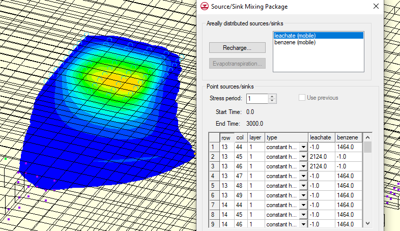
Note that it may seem as though a value of zero would have the same result when defining concentration. However, this is not the case. Entering a value of zero will be recognized as the same as entering a positive value. Therefore, it is important to enter a negative value for species that need to be left undefined when working with a multispecies simulation.

When running MT3DMS, cells that have negative values entered for a species will not have constant concentration for that species applied to that cell. Concentration, constant or varying, will be applied to all cells where the value is positive. As always, it is important to review the entered species values before running the model to ensure accuracy.

Now with more understanding of how to work with constant concentration values for multiple species in MT3DMS, see if you can use it in your GMS project today!

Blog tags:

GMS

New MODFLOW-USG 3D Dataset to Array

By aquaveo on March 26, 2024

While most groundwater projects typically only need a 2D dataset to define arrays, 3D datasets are becoming more available. There’s a new feature in the Ground-water Modeling System (GMS) version 10.8 for MODFLOW-USG and MODFLOW-USG Transport models. MODFLOW-USG and MODFLOW-USG Transport are MODFLOW models that were designed specifically to be used with unstructured grids, or UGrids. The Recharge (RCH), Evapotranspiration (EVT), and EvapoTranspiration Segments (ETS) packages in MODFLOW-USG now have the option to use a 3D dataset to define the input arrays. Previous versions of GMS only had the option to use a 2D dataset with a matching 2D structured grid.

Example of the 3D Dataset to Array option

You can find the 3D Dataset → Array button in the properties dialog of the Recharge (RCH), Evapotranspiration (EVT), or EvapoTranspiration Segments (ETS) package. In order to use the 3D Dataset → Array button, the 3D dataset in the MODFLOW-USG model has to have the same number of rows and columns as the 3D grid. If the rows and columns don’t match the 3D grid, then the button will be grayed out and you won’t be able to use it.

Clicking the 3D Dataset → Array button will bring up a Select Dataset dialog with a list of all the datasets associated with the current 3D grid. You can then select the relevant dataset to assign values to the MODFLOW-USG package. 3D datasets are often created using the 3D Scatter Point tool, which can help you interpolate rainfall data to the cells on your grid. If you are using a transient dataset, then the dataset values will be interpolated linearly to each stress period when they are copied to the array. You can learn more about using the 3D Scatter Point tool on this page of our wiki.

Now head over to GMS 10.8 and try using the new 3D Dataset → Array button in your MODFLOW-USG or MODFLOW-USG Transport project today!

Blog tags:

GMS

Understanding Pass Through Cells

By aquaveo on March 5, 2024

Starting with version 10.8, the Groundwater Modeling System (GMS) has the ability to handle pass through cells in MODFLOW-USG and MODFLOW-USG Transport projects. What are pass through cells? If you have a 3D UGrid with multiple layers, you can have middle layers with pinchouts or other features that cause that middle layer to not extend through the entire range of the other layers. For example, if you have a three-layer unstructured grid with a pinchout in layer two, then you will have an area where the cells of layer one and layer three are supposed to meet. This area where a middle layer is missing for some of the cells is where pass-through cells are needed.

In actuality, there is a thin cell between the layers. Because of this, in areas where a middle layer is missing a barrier would be formed when running MODFLOW-USG. If you don’t want a barrier in that area, then you will need to add a pass through cell to allow water to flow through the area. This means you need to have the Ibound be greater than zero or the water will not be able to pass through the middle layer and create a “no-flow zone.”

By switching between layers you can see which layers have a thickness of zero and which do not. To inactivate the cells with a thickness do the following:

Open the MODFLOW Global/Basic Package dialog.
Select the Set Pass Through… button.
A message will appear explaining parameters used to determine pass through cells.
In the Pass Through Thickness dialog, set the maximum cell thickness.

After assigning the maximum cell thickness, cells that are below that thickness will be designated as pass through cells. The pass through cells will have an inactive IBOUND and will be ignored when making vertical connections in the DISU package.

Note that setting pass through cells requires a stacked grid.

Now that you know about pass through cells, make use of them in your MODFLOW-USG and MODFLOW-USG Transport projects in GMS today!

Blog tags:

GMS

Generating a 3D Grid from Raster Data

By aquaveo on February 13, 2024

Have you heard about the 3D UGrid from Rasters tool that’s new to the Groundwater Modeling System (GMS)? Previous versions of GMS required you to build a raster catalog and then use the “Horizons to Solids” command in order to generate a 3D unstructured grid (UGrid) when modeling stratigraphy. The 3D UGrid from Rasters tool, which is in GMS’s toolbox under the “Unstructured Grids” folder, streamlines this process by allowing the two previously separate processes to be set up in the same place and executed simultaneously.

Example of a 3D UGrid generated from rasters

The base components for creating a UGrid with the 3D UGrid from Rasters tool are a 2D UGrid and multiple rasters. The rasters are then added to a table and assigned a horizon number. The term “horizon” refers to the top of each stratigraphic unit that will be represented in a corresponding solid, HUF unit, or 3D mesh layer. Horizons are ordered from the bottom up. For each raster you can choose to fill or clip the layer. Choosing “fill” tells GMS to use the raster to create a UGrid layer. Choosing “clip” tells GMS that any lower surfaces should truncate at that layer. You also have the option of creating sublayers between any rasters that have the “fill” option turned on. You can then set the relative size of each of the sublayers so that they are all proportional, or of differing sizes.

After setting all of the parameters for your UGrid in the rasters table, you then need to set a target location so that GMS knows to calculate elevations at the UGrid cell tops and bottoms or at the points. Lastly, you’ll need to define the minimum thickness that every layer must have, and choose a name for your new UGrid.

If you want more details about how the 3D UGrid from Rasters tool works, you can check out this page of our wiki. You can also look at the newest version of the Horizons with Rasters tutorial.

Head over to GMS, and use this new tool to simplify the stratigraphy modeling process.

Blog tags:

GMS