Aquaveo & Water Resources Engineering News

Viewing SRH-2D Simulation Plots

SMS generates multiple plots during the SHR-2D model run. These solution plots include data collected by monitor points or lines as well as information such as mass balance and percentage of flow that enters the simulation. This post will discuss accessing and using the solution plots.

The first way to view the SRH-2D Solution plots is through the simulation data in the Simulation Run Queue. This allows you to look at the quality of the simulation as it is running. In the Simulation Run Queue, the Monitoring data option needs to be turned on. You can then view the plots as they are generated using the tabs below.

After you have run the simulation, you can view the solutions plots. You can access the SRH-2D Solution Plot by doing the following:

  1. Right-clicking on the simulation item and select Tools from the dropdown to open another submenu.
  2. Click on View Simulation Plots to pull up the SRH-2D Solution Plots window.

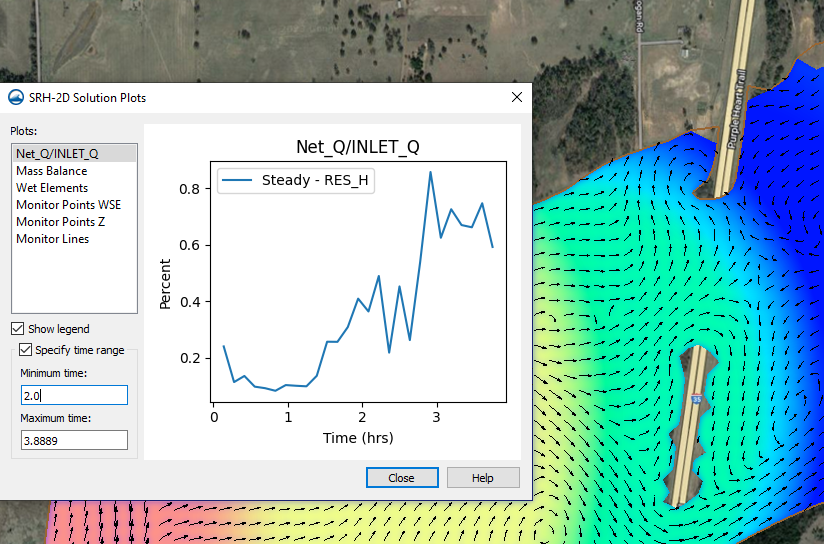
This will allow you to look at the list of different plots in the Plots section. On the left, there are a few other options such as the legend, and specifying the time range. The show legend option will have a legend appear in the upper right corner of the plot that has been pulled up. This as well as the specifying of the time range allows you to adjust the graph to your desired time range.

Example of the Solution Plots dialog

It is important to note that the plots in the Solution Plot window are not available in the Plot Wizard. You will need access them through the Solution Plots window. With that, it should be noted that pulling up an older SRH-2D project in a current version of SMS may not have the solution plots. This is because of changes in how files are organized. In this case, the solutions plots can be generated by re-running the simulation.

The SRH-2D Solution Plot is one of the many options in SMS to help you see what is happening in your simulation. Try using the SRH-2D Solution Plot in SMS today!

Blog tags: 

Working with Inactive Cells in MODFLOW 6

When working with a MODFLOW 6 model in the Groundwater Modeling System (GMS) it can be important to mark specific cells inside a project as inactive to keep it out of the computational domain. Using inactive cells can speed up the performance and accuracy of your model. Incorrectly designating cells as inactive or active can cause inaccuracies in your model or keep it from converging. Here is some guidance for working with inactive cells that will help create a better MODFLOW 6 model.

Modflow 6 model with inaccurate z values

When choosing which cells to mark as inactive in GMS, it is helpful to know how to find information about the cells in the first place, as well as what information MODFLOW 6 is using to calculate the X, Y, Z, and S values of that cell. The display above the graphics window that shows the values of the selected cell is using the cell center for its calculated values. If the inactive cells have a low elevation that is inaccurate for the model, it will drag the Z value for the active cells on the edge down to meet the inactive cell. This happens because the outside active cell has nodes in the Z value that still need something to attach to as there cannot be gaps between the nodes. This will distort the cells in unintended ways and create errors in the model.

MODFLOW 6 uses IBOUND to determine which cells to mark as active and which to mark as inactive. Marking a cell with an IBOUND value of zero will make it inactive.

There are a few ways to inactivate cells in a MODFLOW 6 model. The first is to create a polygon that will separate the active and inactive cells. Select the polygon that contains the cells that are to remain active. Go to the Feature Objects menu and select Activate Cells in Coverage(s). This will automatically make any cells that aren’t selective inactive.

The second way is to select a group of cells with the cell selection tool. Then go to the MODFLOW menu | Advanced | Cell Properties… and change the IBOUND dropdown menu to inactive. This will inactivate only the cells that have been selected in the graphics window.

The cells can also be set as inactive by editing the IBOUND Array directly.The IBOUND dialog can be found by clicking on Global Options under the MODFLOW menu. There is an IBOUND button in this dialog window where the IJK coordinates can be set to zero manually.

Making use of inactive cells can improve you MODFLOW 6 model. Try out MODFLOW 6 in GMS today!

Blog tags: 

Announcing WMS 11.2 Beta

Aquaveo is excited to announce the release of WMS 11.2 in beta! WMS continues to provide an all-in-one watershed modeling solution. With the release fo the WMS 11.2 beta, we want to highlight some of the new features you can find in WMS 11.2 beta.

WinTR-20 Model

WMS 11.2 has improved the use of the TR-20 model by incorporating the WinTR-20 numeric model. WinTR-20 uses the same interface as TR-20. WinTR-20 contains upgrades to the source code with some changes to the input and output files. These changes have now been incorporated into WMS 11.2 to let you take full advantage of these features.

Export MP4 Files

MP4 files are now the default when exporting animations. You can export the MP4 files directly from the film loop wizard in WMS. MP4 files make sharing animations you’ve created in WMS easier.

The Toolbox in WMS 11.2
Toolbox

WMS 11.2 introduces the Toolbox which contains many tools for manipulating data and geometries. This is reached through the Toolbox macro. Of particular use for WMS projects are the tools related to working with rasters and lidar data allowing to trim, merge, and smooth this data along with many other options. The toolbox also contains many tools for working with coverages and datasets.

Color Ramp Options

The final new feature is the changes to the color ramp options. The color ramp now contains multiple preloaded color palettes. Options have been added to reverse pallets and to save your favorite palettes for easy access in the future. The preloaded palettes can also be duplicated and customized to meet your project's needs.

These are a few of the new features that come out with the release of WMS 11.2. Try out these features and more by downloading WMS 11.2 from the Aquaveo website today!

Blog tags: 

Interpolating Localized Elevation Values

Do you have a Surface-water Modeling System (SMS) project where you need to adjust the elevation values for a small area of your mesh? Some projects require updates to the localized areas of the mesh elevation. It may be that you’ve received updated elevation data for part of the project area, or you discovered a flaw in the elevation data on the mesh. You could manually update the elevation on each node of the mesh, but this could be rather time-consuming. Using the Scatter Module in SMS, you can incorporate the new elevation values into your mesh.

Example of localized elevation data

Ideally, you will be able to obtain correct elevation data that covers the entire mesh domain, which you could simply interpolate over to the mesh. But when you only have updated elevation data for a localized area, you can use this workflow to update the elevation data.

  1. Right-click on the desired mesh and select Convert > Mesh → 2D Scatter.
  2. Name the new scatter set whatever you'd like (or keep the default) and keep all other settings the same.
  3. Choose Scatter | Merge Sets to open the Merge Scatter Sets dialog.
  4. Check the box for each scatter set that you would like to merge.
  5. Make your newer data higher on the list so that it will be given priority. Do so by selecting a scatter set and using the Move up or Move down buttons.
  6. Choose Delete lower priority scatter points and check the box for Maintain triangulation.
  7. If desired, name the new scatter set something other than the default.

This will create a new scatter set that overwrites the old data with the new data.

From here, which course you take will depend on whether you need just the z values to change, or if you need the mesh geometry to change as well.

To only change the elevation values in the existing mesh, do the following:

  1. Right-click on the new scatter set and select Interpolate to....
  2. Check the boxes for the scatter set z or elevation dataset as well as the box for Map Z.
  3. Choose the starting mesh from the list on the right.

To create a new mesh with the new elevation values, do this:

  1. Right-click on the merged scatter set and select Convert > | Scatter → 2D Mesh.
  2. Name the new mesh whatever you like and press OK.
  3. Edit the new mesh as needed.

The Scatter Module in SMS gives you a variety of options for fixing and adjusting elevation data. Try out the Scatter Module in SMS today!

Blog tags: 

Refining Quadtree Grids in SMS

Using the Surface-water Modeling System (SMS), you can model quadtree grids for use with numeric models such as CMS-Flow. Quadtrees are part of the UGrid module in SMS making them a type of unstructured grid. When creating quadtrees in SMS, you can choose to have uniform cell sizes, or you may choose to refine the cells in some areas. When refining a quadtree, there are a couple methods and some tips to keep in mind.

The first method for refinding grid cells in a quadtree is to simply select the cells you want to refine using the Select Elements tool, then right-click and use the Refine Cells(s) command. This will equally divide the cells into smaller, more refined, cells. This method is useful for small-scale refinement in localized areas. However, using this method can be tedious if there are multiple areas on the quadtree that need refinement.

Example of the Quadtree Refinement in GMS

The second method for refining quadtrees is preferred in most cases. This method involves setting refinement parameters in the Quadtree Generator coverage. If you are familiar with SMS’s Cartesian grid generator coverage and mesh generator coverage, you will find that it is similar to both of those coverages.

Like the Cartesian grid generator coverage, the quadtree coverage makes use of a grid frame to define the domain of the generated grid. In the grid frame, you decide the size of the cells in the generated quadtree. It is recommended that this cell size be the largest reasonable cell size for the quadtree grid.

Like the mesh generator coverage, the quadtree generator coverage also makes use of polygons. When you create a polygon on the quadtree generator coverage, you can double-click on the polygon to open the Polygon Attributes dialog. In this dialog you can set the grid cell size for all cells that will be within the polygon.

Using both the grid frame and the polygon attributes, you define how the grid cells are refined for your quadtree with more precision. Try out refining quadtree grid in SMS today!

Blog tags: 

Converting Between 2D and 3D Unstructured Grids

Many projects in the Groundwater Modeling System (GMS) start with an unstructured grid (UGrid). GMS supports both 2D and 3D UGrids. The type of UGrid you will need to use will depend on which numeric model you are using for your project. For this reason you may need to change a 2D UGrid to a 3D UGrid or vice versa. This blog post is going to review some of the tools for converting between 2D and 3D UGrids.

Typically, models like MODFLOW-USG or MODFLOW 6 will require a 3D UGrid. If you only have 2D UGrid data, this may require taking a 2D UGrid and converting it to be a 3D UGrid. Likewise, you may need to convert a 3D UGrid to be a 2D UGrid. This is more often done to correct uses with the 3D UGrid, but also to be able to use the data from the 3D UGrid with other applications.

GMS provides two tools in the Toolbox for changing between 2D and 3D UGrids: the Extrude to 3D UGrid tool and the UGrid 2D from UGrid 3D tool. The Toolbox is accessible through the Toolbox macro and these two tools are located with the Unstructured Grids tools.

Example of the Unstructured Grid tools in GMS

The Extrude to 3D UGrid tool converts a 2D UGrid to a 3D UGrid. The tool will allow you to select a 2D UGrid for extrusion, and then it lets you specify the number of layers and layer thickness for each of the new layers. This will extrude the 2D Ugrid to be a 3D UGrid with the specified number of layers that are at a uniform thickness. If you need layers to be at different thicknesses, you will need to edit the 3D UGrid using other tools in GMS.

The UGrid 2D from UGrid 3D tool will collapse a 3D UGrid to be a 2D UGrid. The tool allows you to select a 3D UGrid then select if the 2D UGrid should be created from the top or bottom of the 3D UGrid layers.

The unstructured grid tools in GMS allow you to have more options with how you work with UGrids and grid data for your groundwater projects. Try out the unstructured grid tools in GMS today!

Blog tags: 

Exploring the Drawing Tools in WMS

When presenting a model in the Watershed Modeling System (WMS), you may need to clearly label locations or structures in your watershed model. For example, you may need a graphic with the names of your watershed branches clearly labeled. The Drawing Tools WMS provides a way to clearly annotate your watershed model. This blog post will cover some of the options and uses for these Drawing Tools.

Example of a drawing objects in WMS

The Drawing Tools contain options to draw objects including lines, rectangles, ovals, and text. When using the object creation tools, WMS provides attributes for changing the drawn object. Using the Select Drawing Object tool, you can double-click on a drawn object to pull-up the attribute options for the object. This includes options to change the line width, color, fill, arrows, and fonts.

It's important to note that drawing objects are layered. The first object you create will be below the next object you create. If you need to change how the objects are layered, the Drawing Tools contain tools for moving the objects forward or backward. To do this, select the object, then use the Move to Back, Move to Front, Shuffle Up, or Shuffle Down options to move the object.

You have the option to set a depth for the objects when creating new drawing objects. This depth is based on the project projection. Using the Drawing Depths command in the Drawing Objects menu, you can set a depth for the object you create. This can help make certain the drawing objects are above the grid, feature objects, or other items in the project.

It is important to note that the drawing objects are attached to the project projections. This means that drawing objects will stay fixed to the location of the model coordinates, not the Graphic Window position. This allows you to pan or zoom around your model and the drawing objects will stay fixed to the model location.

The drawing tools will be included when saving an image of the Main Graphics Window. This allows saving an image with annotations for use in presentation materials. To do this, use the Save As command and select the JPEG Image option for the file output.

The Drawing Tools are one of the options provided by WMS to let you make clear presentations for your watershed models. Try out the Drawing Tools in WMS today!

Blog tags: 

Working with Functional Surfaces for UGrids in SMS

The functional surface option in SMS allows viewing data above a geometry. It has been an option in the 2D Mesh module. The functional surface option has been added for unstructured grids (UGrids) in the UGrid module starting with SMS 13.2. This post will give some guidance and tips for using functional surfaces with UGrids.

Example of a functional surface on a UGrid

Functional surfaces use any dataset as the elevation value for the surface. One of their most common uses is as a representation of the surface of the water above a UGrid. For example, the ocean’s surface in a CGWAVE model. However, functional surfaces can use any scalar dataset to inform the elevations.

A UGrid functional surface gets created by the New Functional Surface UGrid right-click command in the Project Explorer. Once created, right-click on the newly created functional surface to edit the display options. The Functional Surface Options dialog allows you to fine tune the display of your UGrid functional surface. Furthermore, selecting Other Display Options brings up UGrid-style display options.

Once you've set up your functional surface, you may need to make adjustments. Here are some tips on adjusting your functional surface displays depending on your situation:

  • If your dataset has large numbers, your functional surface might be very tall. To temper that effect, you could set the functional surface Z Magnification between 0 and 1.
  • If your dataset has very small numbers, your functional surface might appear completely flat. To more clearly see the rise and fall of the data values, set the Z Magnification to a value greater than 1.
  • If your functional surface is intersecting the UGrid, and you don't want it to, adjust the Elevation Z Offset.
  • If you want to add contours to your functional surface, click Other Display Options and turn on Face contours. Then click Contours to open the Contour Options.
  • If you still want to be able to see the UGrid through the functional surface, adjust the transparency. If you're using contours for the functional surface, you'll need to adjust the transparency in the Contour Options dialog.
  • If you want the functional surface to reference a specific dataset for its elevation, specify a User defined dataset.

Try out functional surfaces with UGrids in SMS today!

Blog tags: 

Using the MODFLOW HFB Package

Sometimes in a MODFLOW simulation, you need to simulate very thin barriers to flow that aren't accurately represented by assigning values to entire cells. Fortunately, MODFLOW has the Horizontal Flow Barrier (HFB) package that facilitates accurately modeling thin flow barriers. Today, we explore how the HFB package can meet your needs, and how it functions.

The HFB package can meet your need for a more realistic approach to simulating horizontal barriers in your model. Whereas many packages in MODFLOW assign values to entire cells, that might poorly reflect reality for horizontal flow barriers with negligible width. These barriers might include slurry walls, sheet pile walls, or diaphragm walls around wells. Instead of assigning values to whole cells, the HFB package uses cell boundaries to simulate horizontal barriers. Doing so can more accurately reflect the actual situation.

To use cell boundaries to simulate horizontal flow barriers, the HFB package uses a hydraulic characteristic. You calculate the hydraulic characteristic by dividing the hydraulic conductivity of the barrier by the real-life width of the barrier. This value is assigned to cell boundaries. Then, MODFLOW uses that value to modify the regular flow between cells. Thus, you get modified flow at the cell boundaries that have a defined hydraulic characteristic.

Example of the HFB Package in GMS

The following is a suggested workflow for using the HFB package:

  1. Make sure that the HFB package is turned on in the MODFLOW Packages / Processes dialog.
  2. Set up a coverage that can include a barrier by checking Barrier in the Coverage Setup. Define the layers that the barrier affects using the Default layer range in the Coverage Setup.
  3. Draw an arc representing the barrier. In the Attributes table for that arc, set its boundary condition to "barrier". Define its Hydraulic characteristic as you have calculated it.
  4. Map from that coverage to MODFLOW.

The values for the HFB package can be edited using the HFB - Horizontal Flow Barrier command in the MODFLOW menu.

While using the HFB package, keep the following in mind:

  • There are certain assumptions that this package uses to function. It's assumed the barrier has no storage capacity. It's also assumed the barrier has negligible width. Therefore, the HFB package's sole function is to reduce conductance between adjacent horizontal cells.
  • This blog post primarily applies to standard MODFLOW versions. The HFB package is also available for MODFLOW 6.

Try out the HFB package in GMS today!

Blog tags: 

Computing a Courant Number for an SRH-2D Model

Sometimes, you might want to calculate a Courant number for your SRH-2D model. In most cases, this isn't necessary because SRH-2D is an implicit model. Unlike explicit models such as HEC-RAS, SRH-2D is not Courant limited. With SRH-2D, it is more important to verify convergence and stability than Courant compliance. However, we know that calculating a Courant number dataset for SRH-2D is occasionally desired. Fortunately, SMS now has the Advective Courant Number tool to compute a Courant number dataset based on velocity.

First, let's be clear about what a Courant number does. A Courant number tells you the number of mesh elements that a given water particle passes through during a time step. If the Courant number is less than one, the given particle of water would not pass through an entire mesh element in a single time step.

In SMS, the Advective Courant Number tool computes a Courant Number dataset including every node at every time step. It uses the following equation:

Courant Number Equation

To use the Advective Courant Number tool, do the following:

  1. Make sure a transient SRH-2D solution file is already loaded.
  2. Open the SMS Toolbox, and under Datasets, find the Advective Courant Number tool.
  3. Set the Velocity dataset, the time step length for the simulation, and the desired name for the output dataset.
  4. Run the tool.
Example of the Advective Courant Number tool

The Advective Courant Number tool might stall depending on the vector dataset for your SRH-2D simulation. Running the SRH-2D simulation again might solve this problem. Before running the simulation again, we recommend saving the project as a new file to preserve the old solution files. Then, in the new SMS project file, run SRH-2D again. Once the new solution is loaded into SMS, run the Advective Courant Number tool again using the new velocity dataset.

To see the results, open the Properties dialog for the Courant number dataset. There, you will find the maximum and minimum for the whole dataset and the current time step.

Calculate the Courant number dataset for your SRH-2D simulation in SMS today!

Blog tags: 

Pages