Aquaveo & Water Resources Engineering News

Using Layer Range Options in GMS

The conceptual model approach in GMS is a very useful way to assign specific attributes to a MODFLOW model without having to manually input them cell by cell. One particularly helpful tool available in a GMS coverage is the "Layer Range" option.

Example of the Coverage Setup for Layer Ranges

Layer range can be used in addition to other coverage choices—such as streams, wells, rivers, head boundary, etc.—allowing you to be as precise as you need to be when applying your model attributes.

In the past, we have mentioned this tool in a blog post about assigning Ugrid attributes to specific layers, but that is only one of many helpful ways to use it. Here, we will go over each of the options available with the Layer Range, and exactly how they work.

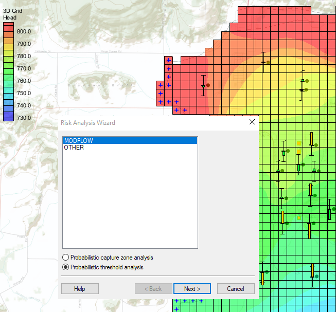
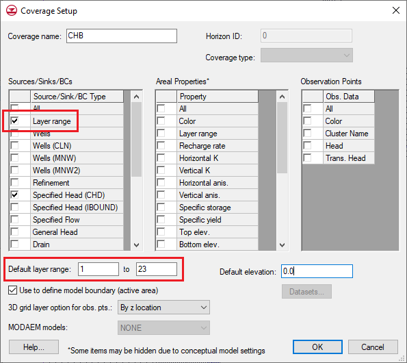
First, turn on this option by selecting "Layer Range" in the sources/sinks column of the coverage setup dialog. At the bottom of this dialog, make sure that the default layer range for the coverage covers all the parts of your grid that you wish to use.

Second, apply feature objects to your coverage. In our example, we have created a Time-Variant Specified Head arc.

Example of the Layer Range Assignment in GMS

Once your feature objects are in place, you can assign values to them in the attribute table. This is where the Layer Range settings will come into play.

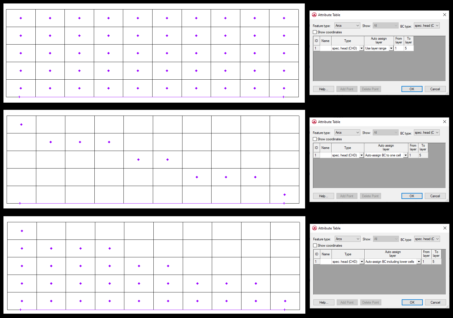
  • Use Layer Range: This option applies your feature objects to a specific range of layers. That range is selected in the attribute table under "From Layer" and "To Layer". A feature point assigned a layer range of 2–6 will be applied to every cell in that vertical column from layer 2 to layer 6.
    Similarly, a polygon or arc will apply its attributes to the whole assigned layer range for every vertical column that it intersects.
  • Auto-Assign BC to One Cell: Any time you want only one cell per column, you can choose "Auto-Assign BC to One Cell". This setting is especially useful when mapping an object type that can't or shouldn't be applied to more than one vertical cell at a time. Stream arcs are one example.
    Auto-assigning to one cell will use the elevation inputs from your feature object to choose the most applicable cell in that vertical column to receive the assigned attributes.
  • Auto-Assign BC Including Lower Cells: This setting allows the coverage to automatically calculate which initial layer the object is applicable to, similar to the "One Cell" option. It then applies the object to that cell, and to everything below it within the range of the coverage.
    Including the lower cells is very useful when you do want more than one vertical cell to be assigned, but need different layer ranges for different parts of the same feature object.

Once you have selected the Layer Range option that best suits your model, you can map the coverage to your simulation. The results can be viewed in the MODFLOW | Optional Packages dialogs, as well as the Sources/Sinks table in the right-click menu for the grid cells.

The Layer Range tool is a great way to get your model attributes as specific as you need them to be without any laborious manual editing. Try it out in your GMS model today.

Blog tags: 

Using the ADCIRC Levee Elevation Tools

Have you needed a way to quickly fix a levee structure in your 2D mesh for your ADCIRC model? The SMS toolbox has tools devoted to helping you develop ADCIRC models that accurately reflect levee elevations. That’s our focus in today's blog post.

The elevations on your levee can affect the outcome of your ADCIRC model. What's more, having the wrong levee elevations can even cause your ADCIRC model to fail its run. But the Check/Fix Levee Crest Elevations tool and the Check/Fix Levee Ground Elevations tool are designed to help mitigate this issue. These tools ensure that the elevations both on the ground and on the crest of your ADCIRC levee feature match the desired measurements.

For example, an ADCIRC model run can fail because the levee ground elevation is higher than the levee crest elevation. The Check/Fix Levee Ground Elevations tool checks the ADCIRC domain elevation against the boundary condition coverage that defines the levees. Then, if adjustments are required, the Check/Fix Levee Ground Elevations tool creates a new dataset that can be mapped as the elevation for the 2D mesh.

On the other side of things, the Check/Fix Levee Crest Elevations tool can help ensure that the crest of the levee in the model does not go above or below the known measurements for the levee crest. A check line is either created in a coverage or imported into SMS then converted to a coverage. The check line has levee crest elevation information against which the Z values of the levee arcs get checked. If the levee crest elevations vary too much from the check line’s elevations, then the Check/Fix Levee Crest Elevations tool adjusts the z values on the levee arcs to match the check line.

Example of the ADCIRC Check/Fix Levee Crest Elevations tool

In short, the Check/Fix Levee Crest Elevations and the Check/Fix Levee Ground Elevations tool can facilitate your modeling of ADCIRC levee features.

Try out these new levee elevation tools in SMS today!

Blog tags: 

Using a 2D UGrid with SRH-2D

A 2D mesh in SMS has long been the standard geometry for SRH-2D simulations. However, you might have noticed in more recent versions of SMS that SRH-2D simulations can also use 2D unstructured grids (UGrids). Today, we examine what using a 2D UGrid can mean for SMS users who model SRH-2D simulations.

Being able to use a UGrid offers a couple advantages. For one, 2D UGrids don't require the SRH-2D Post-Processor because, unlike 2D meshes, they are already centroid-based. This means the SRH-2D results can be read directly onto the 2D UGrid. Additionally, the same SRH-2D model can be run with a mesh and then run with a 2D UGrid. Since the two geometries differ in how they store data, this practice might be helpful in troubleshooting issues with the geometry design for your model. In most cases where the mesh is well built, there should not be significant differences between the results you get from a UGrid-based SRH-2D simulation and a mesh-based simulation.

The steps for creating a 2D UGrid for an SRH-2D simulation are essentially the same as creating a 2D mesh:

  1. Build a mesh generation coverage with polygons.
  2. Specify what kind of grid-like structure you want in each.
  3. Instead of converting the coverage to a 2D mesh, convert it to a 2D UGrid.

An already-existing 2D mesh can also be converted to a 2D UGrid if so desired.

Example of the 2D Mesh Polygon Properties dialog being used for UGrid or mesh generation

It's important to note that there are not yet any manual tools for editing 2D UGrids, so any desired adjustments to a 2D UGrid should be made before the UGrid is generated. As with the 2D mesh, this can be done by double-clicking in the polygons in the mesh generation coverage and using the dialogs that appear.

Furthermore, the principles for creating a quality mesh apply to creating a quality 2D UGrid. The quality of a UGrid is just as important to the model outcome as the quality of a mesh. In 2D UGrids for SRH-2D simulations, please keep in mind the following:

  • The elements should transition gradually from large to small and vice versa. Adjacent elements should not have enormous variations in size.
  • Areas that need more refined results should have finer quality elements.
  • For areas that use the patch option, the elements should be fairly even.
  • Triangular elements should not be excessively narrow.

These are only some of the considerations.

Much of this can be avoided by making sure that the mesh generator coverage is designed correctly. Again, adjustments to the 2D UGrid can really only be made in the mesh generator coverage before the UGrid has actually been generated.

Try using 2D UGrids in an SRH-2D simulation in SMS today!

Blog tags: 

New Features in GMS 10.7 Beta

We are pleased to announce that GMS 10.7 has been released in beta. In order to improve your groundwater modeling projects, we’ve included many new features into GMS 10.7. Here are a few of the new features we are excited about.

Animation Tools Allow Exporting in MP4 File Formats

GMS 10.7 has been improved to allow you to save your animation files in the MP4 format. This will enable you to open animation files outside GMS and view the animation created before returning to GMS. An MP4 file is a common animation file that allows you to open the animation in a number of different player applications.

Introduction of the New Toolbox Features
Example of the Toolbox in GMS 10.7

GMS has added a new Toolbox feature. This Toolbox contains many different tools for completing common calculations and functions in GMS. For example, the new Toolbox contains a tool for merging datasets and another tool for converting geometries to an unstructured grid. We have provided dozens of tools in the Toolbox to work with a wide range of data, so we recommend looking through the available tools to see what would be of most use for your projects.

Many of the tools in the Toolbox can be used instead of using the Data Calculator. This shortcuts some of the processes to help you build your groundwater model faster. Additional tools will be added in future versions of GMS. If you have a common process that you would like to see added as a new tool in the Toolbox, please let us know.

Updated MDT Package for MODFLOW 6

In MODFLOW 6 has updated the MDT package. The MDT package allows for matrix delineation transport as well as shifting matrix delineation start time. Improvements have been made to how this package works with MODFLOW 6 in GMS.

These are just a few of the features that are a part of GMS 10.7 beta. Try out these features and more by downloading GMS 10.7 Beta today!

Blog tags: 

Trimming DEMs in WMS

Have you imported a DEM into WMS but wanted to trim it down to use only a part of the original data? WMS has tools designed to help you trim DEMs that you have imported into WMS, so you can use only the part of the data that's relevant to your model. In this article, we explore the ways that this can be done in WMS.

Trimming a DEM can help eliminate extra data that is not necessary for your project. Having a DEM that is too large or contains data that is irrelevant to your project can cause your project to operate slower and in some cases can skew the results of your project.

One option for trimming a DEM is when it's part of the GIS Data Module as a raster. To do this, draw a feature object polygon in a map coverage then select it. With the polygon selected, you can right-click on the raster and select the Convert To | Trimmed Raster command. This trims the raster along the border of the polygon. The trimmed raster can be converted, if desired, to a DEM that will show up under the Terrain Data folder.

Of course, there are also tools for trimming files that are already in the Terrain Data Module as DEMs. These tools can be accessed either through the DEM menu when in the Terrain Data Module or through the right-click menu for a DEM item in the Project Explorer. In both places, the tools are found in the Trim submenu.

There are two ways to trim DEMs in the Terrain Data Module: by elevation and by polygon.

When trimming a DEM by elevation, WMS brings up a dialog that lets you specify the maximum elevation that you want the DEM trimmed to. The newly created DEM will have only elevations up to the maximum elevation set in this dialog. The contours will likely change to represent the new range of values in the trimmed DEM.

Example of trimming a DEM using a polygon in WMS

When trimming a DEM using a polygon, the program turns the mouse into a tool to click out the polygon in the Graphics Window. To finish the polygon, double-click where the last point is desired. Once the polygon is complete, the trimmed DEM is automatically created.

Note that a DEM created this way is still a rectangle. This is part of the definition of a DEM. However, only the points inside the drawn polygon will be active, so the displayed contours will end at the borders of the polygon you drew. The points that were outside the drawn polygon, which make up the rest of the bounding rectangle, are set to NODATA.

Take advantage of DEM trimming tools in WMS today!

Blog tags: 

The Create Bridge Footprint Tool in SMS 13.2

Do you have an SMS project with a bridge represented in the mesh? SMS 13.2 offers a new tool called Create Bridge Footprint that assists in representing bridge footprints in SRH-2D simulations.

Since the real-life effects of bridges can be complex, creating a mesh to represent them is often challenging. Modeling piers and abutments using older methods in SMS requires many polygons in Mesh Generation coverages. Now, the Create Bridge Footprint tool provides an alternative approach to creating an unstructured mesh under and around a bridge structure. Note that this tool replaces the functionality made available in the Bridge-Piers coverage, which you might have been using in SMS 13.1. However, many of the same settings are incorporated in this tool as well.

The Create Bridge Footprint tool, located in the Toolbox dialog, produces a coverage and mesh that represent the bridge footprint. These features can then be used to create a mesh that incorporates the bridge footprint into the larger mesh for the model.

Example of the Create Bridge Footprint Tool

The set up for the tool includes creating a new coverage with arcs that define the new bridge:

  • The first arc should define the centerline of the bridge. It is the longest arc.
  • Other arcs, drawn across the first arc, define where the piers and abutments are located. The length of the piers is set in the tool parameters before the tool is run, so the length of these arcs is unimportant.

When drawing the feature arcs to represent the bridge for the tool, there are some important things to keep in mind. One of them is that the bridge feature arcs must be the only feature objects in the coverage. Any other objects will confuse the Create Bridge Footprint tool.

It's also important to make sure that all of the shorter arcs cross the centerline, but none of them should intersect the centerline. In this case, intersecting is different from crossing in that it creates a node on both arcs. This splits the centerline arc, making it impossible for the tool to interpret the intended meaning of the arcs.

After setting up the arcs, there are some parameters to set in the tool to complete the model of the bridge. Then the tool can be run and the resulting mesh and coverage reviewed, and you're one step closer to completing your model.

Try the Create Bridge Footprint tool in SMS 13.2 today!

Blog tags: 

Using Map from Coverage in GMS

If you are using MODFLOW 6 in GMS, you may notice that it uses a different workflow than other versions of MODFLOW in GMS. These changes were made to improve flexibility and performance for groundwater modeling in GMS. One difference is the process of mapping data from the conceptual model to the MODFLOW simulation. In all versions of MODFLOW in GMS, mapping involves taking data input in the conceptual model and "mapping" that data to the grid or mesh being used by the MODFLOW simulation. With every other version of MODFLOW, this is accomplished using the Map to MODFLOW command. However, in MODFLOW 6, mapping is accomplished using the Map from Coverage command.

Now, why this change? It mostly has to do with differences in how GMS handles these different kinds of MODFLOW. A GMS project can only hold one older MODFLOW simulation, but GMS was improved to allow multiple MODFLOW 6 simulations in a project. For handling multiple models and simulations, the Map to MODFLOW command is insufficient. There might be multiple simulations in your project, and you might not want the coverage or conceptual model you are pulling data from to map to all of these MODFLOW 6 simulations.

So how does the new command work? For a MODFLOW 6 package in GMS, do the following:

  1. Right-click on the simulation package and select the Map from Coverage command.
  2. Select a coverage for GMS to map over the package.
Example of the Map from Coverage coverage

GMS will then map the data from the coverage into the MODFLOW 6 package. It's important to note that only some of the MODFLOW 6 packages can be mapped from coverages. This means some packages must be manually set up in their package dialog. This new workflow can have some important effects on how you build your MODFLOW 6 simulation. In MODFLOW 6 it’s especially important that you map over the correct coverage. Since the data isn’t generically mapped over to MODFLOW, it’s especially necessary to know which coverage will be used to define each MODFLOW 6 package.

Try out the Map from Coverage process for MODFLOW 6 in GMS today!

Blog tags: 

Tips for Modeling 3D Bridges in SMS 13.2

Do you have an SMS 13.2 project that could benefit from using a 3D bridge? Today's blog post covers some things to consider as you model 3D bridges in SMS.

First, it’s important to know that SMS identifies the arc drawn first as the upstream side of the bridge. So the order in which the arcs are drawn affects the final bridge model. However, before the bridge is fully created, it’s possible to switch which side of the bridge is upstream using the Swap Arcs command in the Bridge dialog. Checking that the arcs are assigned to the correct side of the bridge can prevent errors later in the model.

When the bridge is created, it can be imported automatically into the model. So the bridge file is exported from SMS, but then SMS imports it automatically. To import the bridge automatically, select the Add 3D Bridge UGrid to SMS on OK option in the Bridge dialog. This eliminates the need to search for it then import it.

Example of 3D Bridge Modeling in SMS

However, if the 3D bridge file is moved, it's important to keep in mind that two files were created by modeling the bridge: an XMUGRID file and a PRJ file that contains the projection for the UGrid. These files should be kept together.

Finally, modeling piers is sometimes an important part of modeling a 3D bridge. The top and underside of a 3D bridge are defined using XY Series Editors accessible in the Bridge dialog. When defining any elevation changes in the 3D bridge, the distance (x) values cannot be identical to each other. This means it’s impossible to create a precisely vertical slope using this tool. To approximate a vertical slope, first input distance values that are very close to each other (e.g. 79 and 80). Then, pair them with elevation values that reflect the change in elevation.

Please keep in mind that piers used for an SRH-2D pressure flow model should not be modeled using the 3D bridge tool. Piers in that kind of model should be modeled using voids in the mesh.

Use these tips in creating a 3D bridge in SMS 13.2 today!

Blog tags: 

How to Export Contour Lines as Shapefiles in SMS

Have you been wanting to export the contour lines in your SMS project as a shapefile so they can be opened in a different application? SMS allows exporting contour lines as a shapefile. This post will explain how to export contour lines as shapefiles.

Saving your contours as a shapefile requires your project to be set up correctly. Save the contours as a shapefile by doing the following:

  1. Make sure the contours you want to convert to a shapefile are set to Linear in the Display Options. To do so, open Display Options and click on the page for the geometry that has the contoured dataset loaded (e.g. mesh, UGrid, etc.). First, make sure that contours are turned on. Then, click on the Contours tab. In the Contour Method in the top left, make certain the first dropdown is set to "Linear".
  2. Make sure the desired dataset is active in SMS. This can be done by clicking on the dataset in the Project Explorer.
  3. In the File menu, select the Save As command. In the Save as type drop-down menu, select Shapes Files (*.shp). Then navigate to the desired directory. Make sure it's somewhere you will know how to find it. Then click Save.
  4. Once you’ve clicked Save, a dialog opens that gives you options for converting project information to a shapefile. Select one of the contour options. The “Mesh Contours → Arc Shapefile” option is usually best.
  5. Now open your shapefile in the appropriate GIS software. The contour lines will appear as arc lines.
Example of Exporting a Shapefile from SMS

If you encounter issues with the shapefile, start by checking the folder where you saved the file. Make certain that all of the necessary files for the shapefile are there, including a projection file.

Another item to check is that everything you want in the shapefile is displayed correctly in the Graphics Window before you export. Try using the Uncheck All command in the Project Explorer and then checking only the desired geometry. This could allow you to more clearly see the contours as they will appear in the shapefile. You might also consider using the display options to turn off the geometry elements. This would also allow for clearer visualization of the contours. Once you can see the contour lines clearly, use the display options to adjust the contour lines if needed. Finally, there may be some differences between how SMS displays a shapefile and how other GIS applications display the shapefile. Opening the shapefile in SMS can help you determine if this is the case.

Be aware that selecting the Mesh Contours → Polygon Shapefile option when exporting the shapefile causes SMS to create a shapefile with only polygons. This might not accurately reflect the linear contours displayed in SMS since some of them might be only line segments.

Try out exporting contour lines as shapefiles in SMS today!

Blog tags: 

Risk Analysis for Well Groups

In your groundwater model, do you need a way to capture multiple wells for risk analysis? For example, your project might have multiple pumping wells and you would like to see the probabilistic composite capture zone for all wells in the wellfield. GMS provides a way to access the Risk Analysis dialog for refining stochastic modeling results.

Example of the Risk Analysis Wizard in GMS
  1. First open your project in GMS, making sure to select the Plan View and 3D grid module, it will be more difficult to select wells otherwise.
  2. Using the Select Cells tool, drag a box around the entire grid to select all cells in the grid.
  3. Open the 3D Grid Cell Properties dialog and change the value for the MODPATH zone code to a number of your choice.
  4. Select the coverage of the well to make it active. Using the Select Points/Nodes tool, drag a box around the entire project to select all wells in the coverage.
  5. Select Intersecting Objects to open the Select Objects of Type dialog.
  6. Select 3D grid cells from the list and close the dialog. This will select all 3D grid cells that have a well in them.
  7. Open the 3D Grid Cell Properties dialog.
  8. Change the value for the MODPATH zone code to a different number than the one that was used before, close the dialog and save changes. From here, the probabilistic capture zone analysis should be able to run with the well groups setting turned on.

Please note that particles need to leave their original zone to be mapped on the risk analysis results. That is why nothing will show up when all cells were assigned to the same zone. The recommended solution is to change the zone code of just the cells with a well so that as many particles as possible can leave the assigned area.

GMS allows you to be as general or specific as you need when selecting wells for risk analysis. Try out using risk analysis for well groups using GMS today!

Blog tags: 

Pages