Aquaveo & Water Resources Engineering News

Delineating a Floodplain Using a Scatter Point File

Looking for a quick way to delineate a floodplain in your area? WMS provides a way to delineate a floodplain and create a flood impact map quickly, using many different types of data. This blog post will cover how to delineate a floodplain using scatter point data.

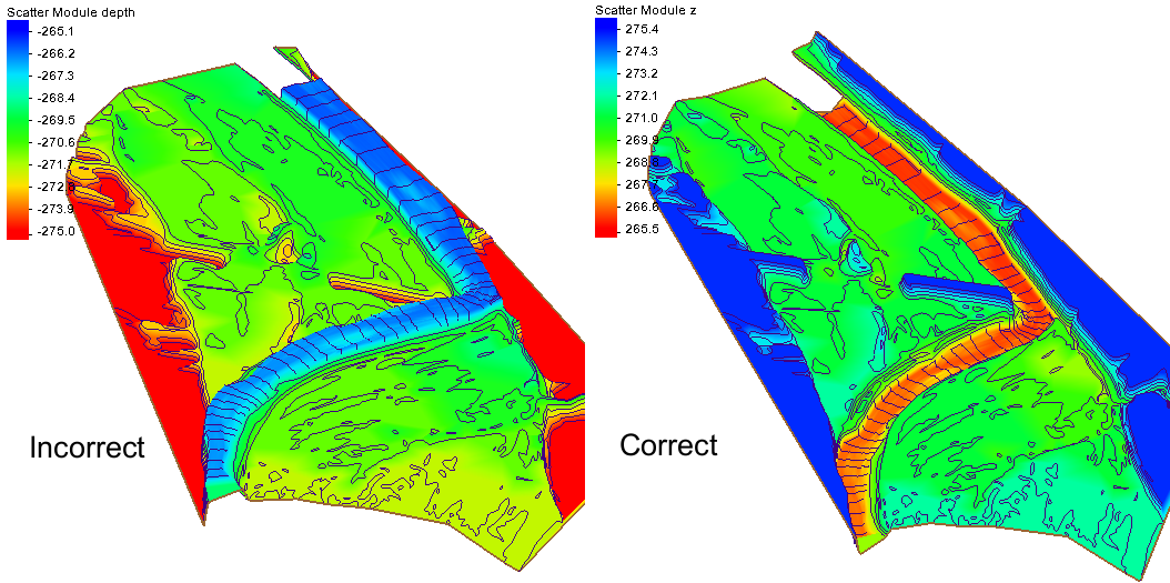
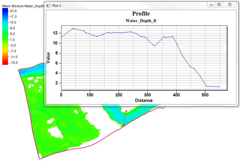
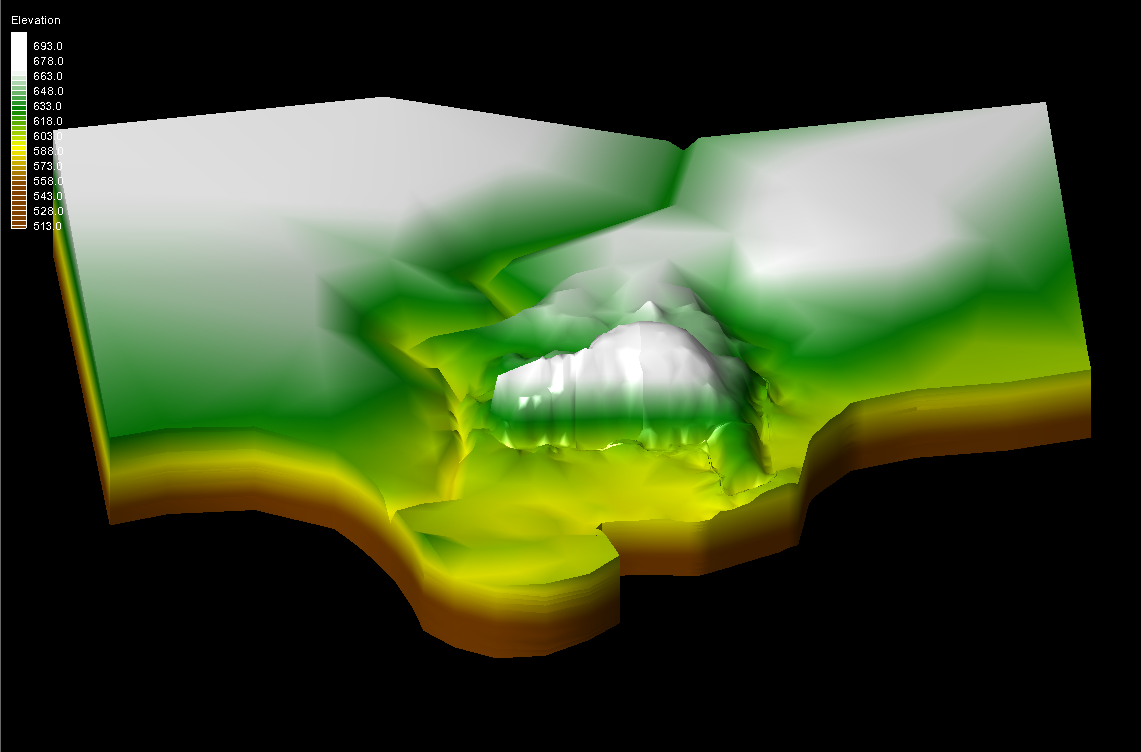
Start by opening your scatter point data:

  1. Use the Flood | Read Stage File menu command to import your scatter point dataset. This is the recommended method for importing a scatter point set for using in delineating a floodplain.
Delineating the Floodplain
flood delineation

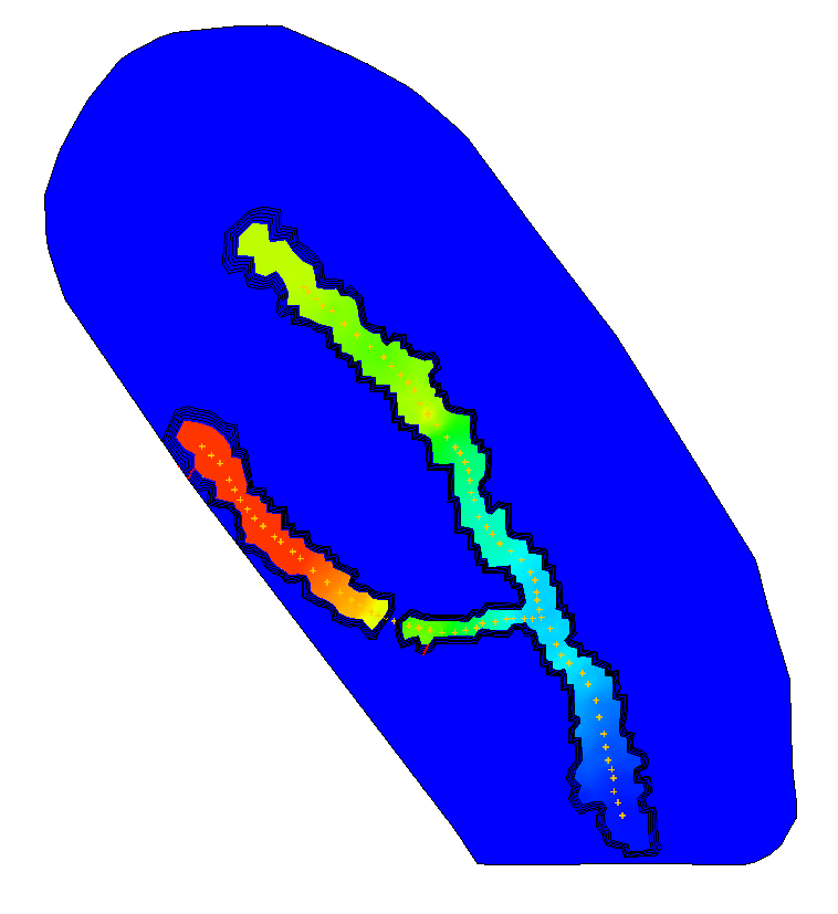
With the scatter point set imported, now delineate the floodplain.

  1. Select Flood | Delineate menu command.
  2. In the Floodplain Delineation dialog, choose the scatter point set you would like to model from the Select stage scatter point set drop-down menu.
  3. Select the specific dataset you would like to delineate from the Select stage data set drop-down menu.
  4. Set options for the Search radius, Flow path, and/or Quadrants depending on your individual model.
  5. When done with the Floodplain Delineation dialog, the delineation process will begin for the set of water surface elevations selected.

In order to create a flood impact map, it will be necessary to have at least two different delineations using varying datasets. If you wish to go on to create a flood impact map, repeat steps 1-5 with a different dataset to obtain a new floodplain delineation.

Creating a Flood Impact Map

WMS can use two separate floodplain delineations to generate a flood impact coverage. A flood impact coverage shows the difference between two flood depth or water level sets. The differences are divided into ranges or classes. Using the floodplains delineated in the previous steps, we’ll create a flood impact map. This can be used to compare how an area will react to a proposed levee for example.

  1. Select Flood | Conversion | Flood → Impact Map menu command.
  2. Choose the Original dataset based off your previous delineations.
  3. Choose your Modified dataset based off your previous delineations as well.
  4. Set the Increase and Decrease sections as desired.

Now that the flood impact map is created, you can use the Select Feature Polygon tool to double click on any of the polygons in the map. This will show you the Flood Extent Attributes dialog, which displays info such as the amount of change between the compared datasets as well as the impact class ID and name.

So this a brief overview of floodplain delineation from a scatter point file using WMS. Try it out in WMS today!

Blog tags: 

Converting Elevations to Depths

Have you ever found that the geometry data you’ve imported into your project is in elevation units, but the model you are using requires depth units? Using the the wrong topographic (elevation) or bathymetric (depth) data type can cause significant inaccuracies in your model results. It can also cause a lot of frustration. Therefore, it is always recommended to ensure you are using the correct data before running your model. SMS provides a way to change your data from elevation to depth (or vice versa) after it has been imported into your project.

Ideally, the correct bathymetry data will be used before assigning it to a geometry (2D Mesh, Cartesian Grid, etc.). When the original bathymetry dataset is incorrect, a new dataset should be created using the correct type (e.g., depth instead of elevation). The Data Calculator allows creating new datasets in SMS. This is done in the Scatter module by doing the following:

  1. Open the Dataset Toolbox
  2. Select the Data Calculator
  3. Select the scatter set
  4. Multiply the scatter set by -1
  5. Compute the new scatter set
  6. Use the new scatter set when generating the geometry
GSSHA

An elevation dataset can also be changed to a depth dataset with an existing geometry that has already been generated. This is done by doing the following:

  1. Open the Dataset Toolbox
  2. Select the Data Calculator
  3. Select the current elevation dataset and add it to the expression
  4. Multiply the dataset by -1
  5. Compute a new dataset

After creating the new elevation set, it needs to be designated as the elevation/depth for the geometry.

  1. Use the Data | Map Elevation command
  2. Select the new depth dataset

Now that you know how to change a dataset from elevation to depth, you can avoid the frustration of having the wrong data in your project. Try out the Data Calculator and other tools in SMS today!

Blog tags: 

Exporting and Importing to MODFLOW 6

In 2018, USGS released MODFLOW 6. This version of MODFLOW uses object-oriented programming to provide support for multiple models within the same simulation. Like many of you, we at Aquaveo were excited to see this new development and started on working on ways for GMS to interface with this new version of MODFLOW.

Did you know that with GMS 10.4 you can export your MODFLOW project for use with MODFLOW 6? This allows you to convert your older or current GMS projects for use with MODFLOW 6. This is just one of the new features in GMS 10.4.

Support has also been added to run MODFLOW 6 from GMS and read the head and flow outputs which may be contoured.

The general workflow process for saving, running, and importing the MODFLOW 6 files is as follows:

  1. After building your MODFLOW model, open the MODFLOW Global/Basic Package dialog.
  2. MODFLOW6
  3. In the dialog, turn on the Save MODFLOW 6 copy option under the MODFLOW Version section.
  4. Save your project.
  5. Open MODFLOW | Advanced | Run MODFLOW Dialog... to run the MODFLOW 6 files.
  6. Use the Custom MODFLOW option to point to the mf6.exe executable in program files (e.g., C:\Program Files\GMS 10.4 64-bit\models\mf6\mf6.exe).
  7. Browse to and select the NAM file out of the *_MODFLOW_mf6 folder that will have saved in the same directory as your GMS project. This is not the default, so you will need to browse for it at least the first time.
  8. Run MODFLOW.
  9. Use MODFLOW | Read Solution to select the MFN file out of the *_MODFLOW_mf6 folder.

The exported files can also be used directly in MODFLOW 6.

In the future, we plan to add more MODFLOW 6 functionality to GMS including a full interface. For now, get ready by converting your projects to MODFLOW 6 using GMS 10.4.

Blog tags: 

New CityWater Pricing

Are you looking at using CityWater? CityWater is a great way to manage water distribution using cloud-based technology.

Recently, Aquaveo changed its pricing system for purchasing a CityWater license. The old system of standard and professional licensing has been modified. When purchasing CityWater, you can now configure CityWater to meet your needs.

Begin by going to the CityWater Pricing page. This page will show you all of the options that can be included in your license. The top of the page shows the core components included in all CityWater licenses. After the core components, a list of components included with each add-on package is shown. Make a note of the add-ons packages needed for your projects and the number of pipes in your largest project before clicking the Configure button.

On the CityWater License Configuration page, you will select the specific features for your license.

GSSHA

Start with entering the number of pipes in your largest EPANET model that will be used in CityWater. This does not limit the number of models that can be uploaded into CityWater, only the size of model. For example, if your largest EPANET model contains 1500 pipes, you could upload any number of models that contain 1500 pipes or fewer.

If later you find that you need to upload a larger model, contact Aquaveo to receive a quote for adding a larger model.

After entering the number of pipes for your largest model, you can select the packages to add to the license. The components of each package are described in the previous page. If later you discover you need a package that wasn’t originally purchased, contact Aquaveo to receive a quote.

Finally, if you are interested in purchasing an Enterprise License of CityWater, you will need to contact Aquaveo for a customer quote. The price for an Enterprise License depends on the number of additional licenses you will be acquiring and the components of each of those licenses.

When configuring your license, the Subscription Summary will automatically update with a quote based on the number of pipes in your largest model and the selected packages. Clicking Add to Cart will take you to the final page where you can review and pay for your order.

If you have any questions about purchasing CityWater or how CityWater can help you, don’t hesitate to contact us at sales@aquaveo.com.

Blog tags: 

Using the Channel Calculator in WMS

With WMS there is no need to sit and calculate your channel properties by hand, you can use the Channel Calculator to help you obtain the hydraulic data you need. The Channel Calculator, a function of the Hydraulic Toolbox, has the ability to give values for flow, depth, area of flow, wetted perimeter, hydraulic radius, average velocity and so much more. Even better, the Channel Calculator only requires some basic cross-section data including the slope and either the flow or depth of the channel.

This blog post will cover how to compute depths for your channels, which can be used to create floodplain delineation maps, and also how to generate rating curves for your channels, which can be used for things such as predictions. To get started, make sure you have cross-section arcs and river centerlines in your model.

To Compute Depths:

The Channel Calculator is a good tool for approximating channel flows or flow depths. Given a flow rate, the Calculator can compute a flow depth, and vice versa.

  1. In the Hydrologic Modeling Module, select Calculators | Channels to open the Channel Calculations dialog.
  2. Toggle on the Use Cross-Section Database option to enable the ability to import existing cross-section data.
  3. Click the Select Cross Section button to bring up the Assign Cross-Section dialog.
  4. Select your cross-section file along with the cross-section you would like to work with.

The cross section displays in the small graphics window of the Channel Calculations dialog. Adjust the Z scale using the drop-down menu to better visualize the cross section. With the cross section selected, set the necessary parameters to perform calculations for depths.

  1. Click the Launch Channel Calculator button to open the Channel Analysis dialog.
  2. Enter a value for Longitudinal slope. This is an estimate for the ground slope in the vicinity of your cross-section.
  3. Enter a value for the Flow or the Depth depending on which values you have and which ones you are trying to find.
  4. Select the Calculate button. This will populate the right-side of the dialog with hydraulic values calculated for the cross-section.
  5. Select the Create Stage Point button in the Channel Calculations dialog to create a stage point based off the values computed in the channel calculator. This is useful if you are planning to use the depths to delineate a floodplain later on.
To Generate a Rating Curve:

The Channel Calculator can also be used to create different rating curves, to be used to calculate things such as storage potential.

  1. Click on the Launch Channel Calculator button to open the Channel Analysis dialog.
  2. Select the Compute Curves button to open the Curve Selection dialog.

The default is to create a rating curve for the entered flow vs. depth for the selected cross section, but it’s possible to also create curves for all of the other options listed.

  1. When exiting the Curve Selection dialog, the selected rating curves are generated and the plot shouldappear.
  2. If you double-click in the rating curve plot window a dialog will appear that presents many different options for how you can use the rating curve, including an option to export the curve in a chosen format.

As you can see, with just a few steps, you can obtain the hydraulic data you need for your channels in WMS. Try it out today!

Blog tags: 

Saving Plots in SMS

After working to put together the perfect plot for your model to show what is going on, it’s nice to be able to keep that plot. Starting in SMS 13.0, you can save plot parameters with your project or for use in other projects.

Previously, SMS allowed exporting the plot as an image or text file, but it did not allow you to save a plot file that SMS could read to regenerate the plot in your project. Saving a plot allows the plot parameters to be used over and over again, saving you from needing to recreate the plot in the future.

To save a plot, do the following:

  1. After generating a plot, use the File | Save As command.
  2. In the Save As dialog, change Save as Type to “Plot File (*.plt)”.

Furthermore, if a plot window is open in SMS when you save your project, a PLT file will be generated to go with your project.

The PLT file that is generated can be opened in any instance of SMS. The file records the parameters used to generate the plot such as the selected datasets, observation arcs used, and plot display options.

GSSHA

Once the plot file has been saved, opening the file in SMS will regenerate the plot. SMS will attempt to recreate the conditions that existed in SMS when the plot was first saved. If the plot is imported into the same project where it was generated, it should appear the same.

If the plot is imported into a different project, SMS will try to match the conditions as closely as possible. For example, if the plot uses an observation arc, SMS will use the first observation arc it can find. If a mesh was used, then SMS will look for the same mesh. It will also look for the same dataset and if it cannot find it, then it will look for a dataset with the same name.

Test out saving plots in SMS 13.0 today!

Blog tags: 

Creating a Confined Aquifer

Does your MODFLOW model contain a confined aquifer? A confined aquifer layer is defined as "an aquifer below the land surface that is saturated with water. Layers of impermeable material are both above and below the aquifer, causing it to be under pressure so that when the aquifer is penetrated by a well, the water will rise above the top of the aquifer."

GSSHA

In MODFLOW, a layer is considered confined when the head in the cell is above the top of the cell. Additionally, any cell located above the water table will be unconfined because the head in those cells will be below the top of the cell.

The layers in your GMS MODFLOW model can be assigned as confined or convertible in any of the flow packages, such as in the LPF package. Other flow packages can be used as well, including the BCF, HUF, and UPW packages. When setting up the MODFLOW model, select the desired flow package in the MODFLOW Packages dialog. The selected flow package must be compatible with the specified MODFLOW version.

In any of the flow package dialogs, under the Layer Type subheading, a layer can be defined as "Confined" or "Convertible". "Convertible" means GMS will automatically assign the layer as confined or unconfined depending on the elevation of the water table in the simulation. Only one layer type can be assigned to each layer. By default, all layers are set to convertible unless specified otherwise.

When a layer is explicitly set to be confined, MODFLOW will use the thickness of the cell, rather than the saturated thickness, to compute a transmissivity value. It will not check for the unconfined condition in the layer.

After defining the layers as confined or convertible, you will have a confined aquifer for your simulation. Try using confined aquifer layers in your GMS models today!

Blog tags: 

Using GSSHA Group Files in WMS

GSSHA Group files in WMS allow multiple GSSHA projects to be saved together in one set of files. It can sometimes be helpful for you to run GSSHA on multiple related projects in order to compare the results.

GSSHA

You can open multiple projects into one WMS session by doing the following:

  1. Open the first project using the GSSHA | Open Project File option.
  2. Open the second, third, ect., project using the same menu.

Once the desired projects are open in WMS, you can save them as a GSSHA Group Project (GGP) file. This keeps everything together in one location.

  1. Save the project as a group by using the GSSHA | Save Group option.
  2. Select the projects to include in the group.
  3. Give the group a file name.

GSSHA can be run on a group file if you do the following:

  1. Select the GSSHA | Run GSSHA Group option.
  2. Select the projects to run.
  3. Give the project a name.
  4. Select whether to suppress screen printing and/or to import the solutions when the GSSHA run finishes.

When GSSHA finishes running on the first project, the Model Wrapper dialog will automatically close. A few moments later, another instance of the Model Wrapper dialog will appear as GSSHA runs on the second project. This one will also automatically close. This continues this way through all of your selected projects. WMS will then import the solutions from the GSSHA runs.

All of the tips here require you to be in the 2D Grid Module—there are additional GSSHA menus in other modules. Additionally, warnings may appear asking if land use and soil type tables should be overwritten. This is up to your discretion. Keep in mind, however, that it is generally best to import projects in an additive manner, with the most simple project being imported first and the most complex project being imported last.

Try out saving and running GSSHA groups in WMS today!

Blog tags: 

How to Relax or Refine a Mesh in SMS

Are you ever tempted to refine your mesh after creation using the mesh editing tools? Manually changing hundreds or thousands of mesh elements using the mesh tools can be very time consuming.

Although possible to use the mesh tools, it is better to recreate a new mesh when wanting to refine or relax the elements. This will maintain the accuracy of your mesh, and reduces possible issues that may arise later on in the project due to inconsistencies that editing manually creates.

To recreate a refined or relaxed mesh:

  1. Create a mesh generator coverage.
    1. If the existing mesh was created from a mesh generator coverage, you can use that coverage or a duplicate of that coverage.
    2. If a mesh generator coverage does not exist, you can create a mesh generator coverage by converting the mesh boundary or nodestrings to a new mesh generator coverage.
  2. Go to your mesh generator coverage and redistribute the vertices so that there are either more or less arc segments depending on what you are trying to accomplish with your model. To relax the mesh, fewer arc segments are desired, and to refine the mesh more arc segments are desired.
  3. Assign the desired meshing type (paving, patch, etc.) to the polygons in the mesh generator coverage and set the bathymetry source to use. Be certain to preview how the mesh will generate with the new spacing for each polygon.
  4. Now generate a new 2D mesh using the edited mesh generator coverage.
  5. Add the new mesh to your model simulation and run the model using the relaxed or refined mesh.

Sometimes you might not want to relax ro refine the entire mesh. To only relax ro refine part of the mesh do the following.

  1. Create a new mesh generator coverage.
  2. Create a polygon in the area of the mesh you wish to relax or refine.
  3. Redistribute the vertices along the arcs in the polygon to so there is a great or fewer number of segments along each arc.
  4. Set the meshing type for the polygon and assign it a bathymetry source. Be certain to preview the mesh for the polygon to be certain you are getting the mesh you want.
  5. Generate a new 2D mesh for the area being refined or relaxed.
  6. Select both 2D meshes and merge them together.
  7. Add the new merged mesh to your model simulation and run the model.

Using these steps when editing a mesh can make a huge difference in your model and save you time. Try out relaxing and refining meshes in SMS today!

Blog tags: 

Assigning Elevations in GMS

GMS offers several options for importing, exporting and manipulating elevation data. With so many options, sometimes it can be confusing when choosing which method to use. If you sometimes struggle with elevation data, you’re in luck, because in this blog post we will be exploring different ways that you can utilize your elevation data to accomplish your goals. Listed below are several ways in which you might be interested in using your elevation data.

  • Assigning elevations in the conceptual model (e.g. to drain nodes)

    Using the Select Points/Nodes Tool , double-click on a point/node such as a drain node. This brings up the Attribute Table dialog. Make sure the Feature Type is set to point/node. Here you can set the type of point/node (such as to a drain or a river) and set the bottom elevation. Things such as river arcs and drain nodes require elevations to run the model in MODFLOW.

  • Interpolating scatter sets/rasters to MODFLOW elevations

    Right-click on the scatter set or raster and select Interpolate To and select MODFLOW layers. This will bring up the Interpolate to MODFLOW Layers dialog. Select the dataset you want to interpolate on the left side of the dialog and the layer you would like to interpolate to on the right-side. With both the dataset and the desired layer selected, click Map. This will add the selection to the Dataset=>MODFLOW data queue. Select Interpolation Options if you want to change the interpolation method. Click OK to exit the dialog and interpolate the scatter set to the layer.

  • Making sure nothing in your conceptual model assigns a polygon elevation that would overwrite the interpolated values

    It is important to note that if you have top and/or bottom elevations assigned as areal properties to a polygon, and you map this coverage to MODFLOW, any scatter points or raster elevations previously interpolated to MODFLOW as the top/bottom elevations that lie within the polygon will be overwritten.

  • Pulling datasets out of MODFLOW (e.g. Layer → 2D Dataset) for manipulation and/or use elsewhere

    Another great feature available in GMS is the ability to pull elevations from a MODFLOW layer to create a 2D dataset. This 2D dataset can then be manipulated and/or used elsewhere for various purposes. This can be done in one of two ways; by using the Layer → 2D Dataset option, or by using the MODFLOW Layers to Scatter option.

  • Layer → 2D Dataset vs. MODFLOW Layers to Scatter (preferred)

    It is possible to create 2D datasets from layer arrays in MODFLOW by going to the Global Options in MODFLOW, and selecting the array you want to create a dataset of (starting heads, top elevations, bottom elevations). In the array dialog box select Layer → 2D Dataset or Grid → 3D Dataset. The dataset that this creates will have ids, i, j, and f values.

    The preferred method for creating datasets from MODFLOW layers is by selecting the layer and then selecting Grid | MODFLOW Layers to 2D Scatter Points. In the MODFLOW Layers → Scatter Points dialog, you can select to create scatter points within a selected coverage and chose the desired coverage. If you use this option, there must be a polygon in the coverage for the points to map to. This dialog also gives many other options that are extremely useful and convenient. When using this method, the 2D scatter set will have x and y coordinates and the f value.

As you can see there are several ways for you to take advantage of the many options available in GMS when working with elevation data. Whether building from a conceptual model, or maybe even building a conceptual model from a MODFLOW simulation, there are many ways to use your elevation data in GMS. Practice using your elevation data in GMS 10.4 today!

Blog tags: 

Pages