Aquaveo & Water Resources Engineering News

Taking Advantage of the SRH-2D Channel Calculator

The Surface-water Modeling System (SMS) provides a useful tool that generates an estimated water surface elevation on an "Exit-H" boundary condition in an SRH-2D model. The Channel Calculator in SMS makes it easier to calculate water surface elevation values. It also gives you greater control of over the parameters

When building an SRH-2D model, the exit boundary will need to be defined. A constant elevation is often used, but this can not be sufficient in many cases. The Exit-H boundary condition is a stage type exit boundary where water surface elevation may be given as a constant number or as a stage-discharge or rating curve. The Channel Calculator is used to compute and assign a normal or critical water surface elevation for the outflow boundary condition. It also gives you greater control over the parameters used to determine the outflow conditions.

Example of the Channel Calculator in SMS

The Channel Calculator is accessed through the SRH2D Assign BC dialog. The Populate using Channel Calculator button appears at the bottom of the dialog when "Exit-H (subcritical outflow)" is selected as the BC Type and the Water Surface Elevation option has been determined.

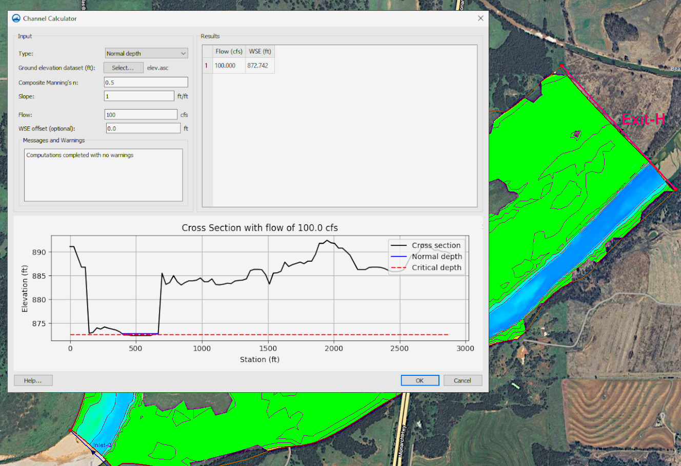
The Channel Calculator specifies a composite roughness value, slope, and flow. SMS extracts a ground elevation cross section from a specified underlying elevation data source (mesh) that is used to compute the area and wetted perimeter. The calculator can make use of different types of elevation data sources which include DEMs, meshes, and scatter sets. Roughness and slope values will be required for the final calculation. Other options, such as the WSE offset, are optional and should only be used when necessary for your project.

The Channel Calculator will display a preview of the exit area cross section with normal and critical depth. When the Channel Calculator will save the values entered when exited. The values in the calculator can be changed later if needed.

The Channel Calculator in SMS gives you a useful tool for determining exit water-surface values for your SRH-2D projects. Try using it in SMS today!

Blog tags: 

Utilizing MODFLOW Symbols Display Options

The Groundwater Modeling System (GMS) has many different options for customizing the display of your project. One display feature created for MODFLOW in GMS is the ability to use symbols to represent the properties of individual cells. This can be quite useful especially for more complicated MODFLOW models. You can use the MODFLOW symbols in the Display Options dialog to represent things like rivers, lakes, wells, drains, and more.

Example of MODFLOW symbols in GMS

You can find the MODFLOW display options as their own tab by selecting the corresponding grid from the list on the left side of the Display Options dialog. The MODFLOW symbols all have a default shape, size, and color. The shape, size, and color of the symbols can all be customized by clicking the button to the left of the checkbox. The ability to customize the MODFLOW symbols is a useful feature for everyone, but especially our users who are visually impaired or color blind. For the best results, the symbols should be set to something different enough from each other that it is easy to tell which is which at a glance.

If you use the MODFLOW symbols in your project, you should consider turning on the display symbol legend. The legend shows a list in the corner of the Graphics Window of all of the MODFLOW cell properties contained within the current project, making it easier to keep track of what everything means. Only symbols that exist in the layer being viewed will appear in the legend.

There are a few additional symbol display options for MODFLOW on the Map Data section of the Display Options dialog. A list of the symbols appears when MODFLOW is selected from the Coverage dropdown. These symbols are specific to properties on the coverages in your project, and they can be customized in the same way as the symbols under the MODFLOW tab of the grid in the Display Options dialog.

Open GMS and use the MODFLOW symbols in the display options to help you keep track of the properties of your MODFLOW project today!

Blog tags: 

Moving Data to Other Geometries

After you have created a model in the Surface-water Modeling System (SMS), it is not uncommon to need to move your vector data or solution datasets from one geometry to another. It could be that your model ran using a 2D mesh and now you want to move the vector data to an unstructured grid for use in another simulation. SMS gives you the ability to accurately move vector data from one geometry to another which can significantly enhance the precision of your modeling efforts.

The Interpolate to UGrid tool is a powerful feature designed to streamline this process of moving datasets from one geometry to another. The Interpolate to UGrid tool is located in the Toolbox with the suite of dataset tools.

Example of the Interpolate to UGrid Tool in SMS

The Interpolate to UGrid tool facilitates the interpolation of a dataset associated with one geometry to another within the same project. While it primarily is meant to work with unstructured grids (UGrids), it can be used with other geometries such as 2D meshes or Cartesian grids. The tool will accept any dataset on the geometry, including vector and elevation sets.

The tool will follow an interpolation process to assign values on nodes or cells from one geometry to the next. Because of this, it is important to review the dataset after it has been moved, to verify that it transferred as expected.

The Interpolate to UGrid tool gives you several features that let you control the process of moving data from one geometry to another. These include:

  • Versatile Interpolation Methods: Choose the interpolation method that best suits your data and modeling objectives to achieve optimal results.
  • Customizable Interpolation Dimension: Tailor the interpolation process to match the dimensions of your target grid, whether it's 2D or 3D.
  • Truncation Options: Control the range of interpolated values with flexible truncation options. Whether you want to preserve the original data range or define custom minimum and maximum values, this tool provides the flexibility you need to fine-tune your results.
  • Extrapolation Capabilities: Handle extrapolation scenarios with ease, choosing from various extrapolation options to extend your dataset beyond the convex hull of the scatter point set.

Whether you're working with unstructured grids, 2D meshes, or other geometric entities, this tool provides the functionality and flexibility you need to enhance the accuracy of your modeling efforts. Make use of the Interpolate to UGrid tool in your SMS projects today!

Blog tags: 

New Import and Export Curvilinear Grid Tools

There are two new tools in the Surface-water Modeling System 13.3 toolbox. If you work with curvilinear grids, then you’ll be pleased to know that there are now tools to import and export curvilinear grids. Both of these tools can be found in the Unstructured Grids folder in the toolbox.

Curvilinear grids are comprised of nodes organized into cells, which define the computational domain of a numerical model. Apart from defining the domain, these grids can also hold extra data like material properties for elements and boundary conditions for nodes. Curvilinear grids must be made up of only quadrilateral elements. This means that if you're creating a grid in SMS, you should make sure you're using the patch method for mesh generation.

Example of the Curvilinear Grid Tools in SMS

There are two file types that are supported for importing or exporting a curvilinear grid: CH3D (also referred to as GSMB) or EFDC (also referred to as LTFATE). Both file types include a cell i-coordinate and a cell j-coordinate dataset option. The EFDC file format includes additional input parameters for a depth dataset, Z roughness dataset, vegetation type dataset, and wind shelter dataset.

The Export Curvilinear Grid tool generates a curvilinear grid file (or files) for a curvilinear compatible mesh, scatter set, or UGrid within SMS. It can utilize user-provided I, J index datasets if available, and offers the capability to calculate I, J data indices. When computing these indices, the orientation of the initial cell on the surface determines the orientation of the grid's I, J axes.

You can use the Import Curvilinear Grid tool to import a pre-existing curvilinear (boundary fitted) grid into SMS as a UGrid object. This process simultaneously generates cell-based datasets that delineate the I, J indices for each cell within the UGrid. The exact format chosen and the nature of the data file(s) selected influence this import procedure.

Head over to SMS and give these new curvilinear grid tools a try!

Blog tags: 

Defining Constant Concentration for Multiple Species in MT3DMS

Are you struggling to define separate constant concentrations for different chemicals in your MT3DMS model areas? MT3DMS is an invaluable tool for groundwater modeling, but like any software, it has its limitations. The Groundwater Modeling System (GMS) incorporates MT3DMS into its interface, which includes both the benefits and limitations of MT3DMS. The inability of MT3DMS to define separate constant concentrations for different chemicals in the same area can be a hindrance for modelers aiming for precision and accuracy in their simulations. So what should you do if your MT3DMS model requires defining constant concentration for two or more chemicals in separate areas?

There's a workaround provided by the MT3DMS developers for defining multispecies simulations. By using negative values in the table for species that need to be left undefined, you can effectively overcome this constraint and tailor your model to your specific needs. In GMS, this value is entered on the Source/Sink Mixing Package dialog for MT3DMS.

Example of the Constant Concentration Settings for MT3DMS

Note that it may seem as though a value of zero would have the same result when defining concentration. However, this is not the case. Entering a value of zero will be recognized as the same as entering a positive value. Therefore, it is important to enter a negative value for species that need to be left undefined when working with a multispecies simulation.

When running MT3DMS, cells that have negative values entered for a species will not have constant concentration for that species applied to that cell. Concentration, constant or varying, will be applied to all cells where the value is positive. As always, it is important to review the entered species values before running the model to ensure accuracy.

Now with more understanding of how to work with constant concentration values for multiple species in MT3DMS, see if you can use it in your GMS project today!

Blog tags: 

Streamlining Watershed Analysis with AGWA

If you work with GSSHA, then you'll definitely want to check out the Automated GSSHA Watershed Analysis, or AGWA, app. AGWA is an online web application for managing proposed changes to watershed models. The app is powered by GSSHA--a hydrologic model developed by the U.S. Army Corps of Engineers.

Example of the AGWA Workflow

AGWA is web-based and therefore can be used from anywhere as long as you have an internet connection and a web browser. It includes simple step-by-step workflows to help you break down a more complex watershed analysis. These workflows can be applied to any number of GSSHA projects. The current workflows include:

  • Detention Basin Analysis
  • Culvert Resize Analysis
  • Find Discharge Tool
  • Land Use Change Analysis

AGWA uses the Tethys platform for managing accounts and access to projects. The GSSHA Models page in AGWA shows a list of all the GSSHA projects that are available for your account. The list includes the project name, project creator, description, and date of creation for each project. You can also view details about the model or the model map from the GSSHA Models page.

Clicking the launch button next to a GSSHA project on the GSSHA Models page will take you to the Model Summary page, which includes two tabs: the Summary tab and the Workflows tab. The Summary tab shows a summary of the GSSHA model including the name and description, map preview, creation date, and a list of scenarios. The Workflows tab shows all workflows that have been created or started, and is where you can create a new workflow.

All completed AGWA workflows have options to view the output data as plots. You can also download the flow and time series data as a CSV file so that you can use the results of your finished workflow outside of AGWA.

Check out AGWA, the app that lets you use GSSHA from anywhere! Follow this link to see a more complete list of the components of AGWA.

Blog tags: 

Tool to Fill a Hole in an Unstructure Grid

Have you ever found yourself working on a mesh in the Surface-water Modeling System (SMS) that has holes in places you don’t want them? Then you may want to check out the new Fill Holes in UGrid tool in the SMS toolbox. This tool can be a quick and easy way to fill in any undesirable voids in your 2D mesh or unstructured grid (UGrid).

Example of a UGrid before using the Fill UGrid tool

The Fill Holes in UGrid tool can be found in the SMS toolbox under the Unstructured Grids folder. From there, all you need to do is select the mesh or UGrid that has holes or voids you want filled from a dropdown list, give the new mesh a name, and run the tool. From there, SMS will create a duplicate of the input mesh, only now the mesh will have elements where the holes used to be.

Example of a UGrid after using the Fill UGrid tool

But what if you want to keep some of the voids in your mesh? That’s where the Extract Subgrid tool comes in handy. The Extract Subgrid tool can isolate a portion of a mesh, which is useful if the mesh is particularly large, or if you want to confine any changes to one specific area.

To create a subgrid, first you need to create an Area Property coverage with a polygon outlining the area you want to isolate. Then open the toolbox and find the Extract Subgrid tool, which is located in the Unstructured Grids folder. Select the mesh from the “Grid” dropdown, the coverage from the “Subgrid boundary coverage” dropdown, and enter a name for the new mesh. Now you can use the Fill Holes in UGrid tool to fill the voids in just the isolated portion of the mesh.

If you use the subgrid method to fill the voids in your mesh, there is one more tool you’ll want to know about: the Merge 2D UGrids tool. You can use this tool to merge the subgrid back with the original mesh. This tool is also in the toolbox under the Unstructured Grids folder. To use this tool, select the subgrid from the “Primary grid” dropdown, the original mesh from the “Secondary grid” dropdown, and choose a name for the new mesh.

The Fill Holes in UGrid, Extract Subgrid, and Merge 2D UGrids tools can help simplify and smooth the mesh editing process, no matter the project. Open SMS 13.3 and check out what these three tools can do for you today!

Blog tags: 

New MODFLOW-USG 3D Dataset to Array

While most groundwater projects typically only need a 2D dataset to define arrays, 3D datasets are becoming more available. There’s a new feature in the Ground-water Modeling System (GMS) version 10.8 for MODFLOW-USG and MODFLOW-USG Transport models. MODFLOW-USG and MODFLOW-USG Transport are MODFLOW models that were designed specifically to be used with unstructured grids, or UGrids. The Recharge (RCH), Evapotranspiration (EVT), and EvapoTranspiration Segments (ETS) packages in MODFLOW-USG now have the option to use a 3D dataset to define the input arrays. Previous versions of GMS only had the option to use a 2D dataset with a matching 2D structured grid.

Example of the 3D Dataset to Array option

You can find the 3D Dataset → Array button in the properties dialog of the Recharge (RCH), Evapotranspiration (EVT), or EvapoTranspiration Segments (ETS) package. In order to use the 3D Dataset → Array button, the 3D dataset in the MODFLOW-USG model has to have the same number of rows and columns as the 3D grid. If the rows and columns don’t match the 3D grid, then the button will be grayed out and you won’t be able to use it.

Clicking the 3D Dataset → Array button will bring up a Select Dataset dialog with a list of all the datasets associated with the current 3D grid. You can then select the relevant dataset to assign values to the MODFLOW-USG package. 3D datasets are often created using the 3D Scatter Point tool, which can help you interpolate rainfall data to the cells on your grid. If you are using a transient dataset, then the dataset values will be interpolated linearly to each stress period when they are copied to the array. You can learn more about using the 3D Scatter Point tool on this page of our wiki.

Now head over to GMS 10.8 and try using the new 3D Dataset → Array button in your MODFLOW-USG or MODFLOW-USG Transport project today!

Blog tags: 

Differences Between AHGW and AHGW Pro

The Arc Hydro Groundwater tools developed by Aquaveo help you manage groundwater and subsurface data within ArcGIS. When ESRI released ArcGIS Pro as the successor to the ArcGIS Desktop applications, we made some changes to the AHGW tools to adapt to the interface of the new ArcGIS application. Today we’ll talk about some of the differences you should expect when making the switch to AHGW Pro. If you're curious about ArcGIS Pro in general, you can follow this link to learn more about it.

Example of the AHGW Pro ribbon

One of the major visual differences between AHGW in ArcGIS Desktop and ArcGIS Pro is the location of the tools. All the AHGW tools in ArcGIS Desktop are located on an AHGW toolbar that can be either docked or floating. In ArcGIS Pro, the AHGW toolbar has been replaced with an AHGW Pro ribbon which includes only some of the tools that were on the old AHGW toolbar. The rest of the subsurface and groundwater analyst tools are imported as a python toolbox. Additionally, AHGW wizards have been converted to panes, which contain all pages of the wizard.

Some of the tools that were previously available in the AHGW desktop applications are not available in AHGW Pro. Some of these tools will be included in upcoming iterations of AHGW, but there are some that will get left behind. Most notably, we have no plans to include any of the AHGW MODFLOW analyst tools in ArcGIS Pro. You may also notice that other file import and export options have been removed.

We made functional changes to some of the AHGW tools in ArcGIS Pro as well. AHGW Pro has moved away from using raster catalogs, using mosaic datasets instread. This may be a little confusing at first, as the tools still have "raster" in the name. Just know that when it says raster, it means mosaic dataset. There are lots of tools that can help you create and modify mosaic datasets inside of ArcGIS Pro, which you can easily find just by typing "mosaic dataset" in the search bar at the top of the window.

Go to ArcGIS Pro and check out the new AHGW Pro tools today!

Blog tags: 

Using the Mask Subset Smoothing Option

The Surface-water Modeling System now includes two new tools in the toolbox to help you when your project requires any amount of dataset smoothing. Previous versions of SMS had you use the Dataset Toolbox to smooth a dataset. These new tools can do everything that the Dataset Toolbox used to do, and more.

Both the Smooth Datasets and Smooth Datasets by Neighbor tools are used to eliminate extreme slopes in a dataset, but they require different inputs, which will tell SMS how to incorporate the relationship between nodes. The Smooth Datasets tool uses an anchor and either an elemental area change or maximum slope for its calculations. Smooth Datasets by Neighbor uses the relationship between neighboring nodes and a selected interpolation method: average or inverse distance weighted. Note that the current version of these tools are designed to be used on node-based datasets, so they will only work on a mesh.

Both of the dataset smoothing tools have the option to include a subset mask. A subset mask dataset is great if there are nodes or elements in your mesh that you don't want included in the smoothing process. Here's some things you need to know when using a subset mask in your project.

Before you begin making changes, your subset mask dataset needs to have the same number of values in the same locations as the dataset being smoothed. A simple way to do this is to right-click on the original dataset in the Project Explorer and select Duplicate. Then you can make changes to the duplicate to create your subset mask dataset.

Example of using the mask subset option

All the nodes you want to have included in the smoothing process need to be set to an S value of "1.0", and the nodes that should be excluded need an S value of "0.0". You can do this in any way you'd like, as long as all nodes get assigned one value or the other. There is a quick method that you may consider using to assign these values. With the Select Mesh Node tool active, right-click in the Graphics Window and choose Select All. With all nodes selected, enter either "1.0" or "0.0" in the S value field depending on whether the majority of nodes should be included or excluded. Then manually select the nodes that should be excluded from the smoothing process by either clicking and dragging a box around the nodes, or by holding down the Shift key and selecting nodes, so that you can select multiple nodes at the same time.

Now this dataset is ready to be used as a subset mask. Open the tool's dialog and select the dataset from the Subset mask dataset dropdown in the tool dialog and enter any other necessary inputs, then run the tool.

To see all the changes, go to the Data menu, select Map Elevation, and select the new smoothed dataset. This will apply the changes that the smoothing tool made to the mesh in the Graphics Window.

Head over to SMS and try including a subset mask dataset with the Smooth Dataset tool today!

Blog tags: 

Pages