GMS

New Features in GMS 10.7 Beta

By aquaveo on September 14, 2022

We are pleased to announce that GMS 10.7 has been released in beta. In order to improve your groundwater modeling projects, we’ve included many new features into GMS 10.7. Here are a few of the new features we are excited about.

Animation Tools Allow Exporting in MP4 File Formats

GMS 10.7 has been improved to allow you to save your animation files in the MP4 format. This will enable you to open animation files outside GMS and view the animation created before returning to GMS. An MP4 file is a common animation file that allows you to open the animation in a number of different player applications.

Introduction of the New Toolbox Features

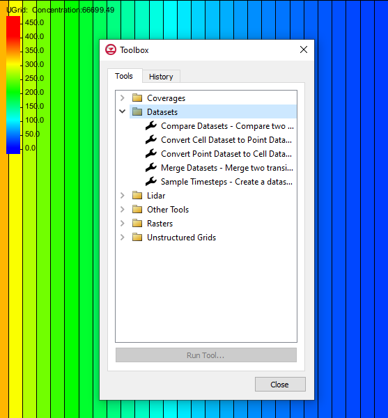
GMS has added a new Toolbox feature. This Toolbox contains many different tools for completing common calculations and functions in GMS. For example, the new Toolbox contains a tool for merging datasets and another tool for converting geometries to an unstructured grid. We have provided dozens of tools in the Toolbox to work with a wide range of data, so we recommend looking through the available tools to see what would be of most use for your projects.

Many of the tools in the Toolbox can be used instead of using the Data Calculator. This shortcuts some of the processes to help you build your groundwater model faster. Additional tools will be added in future versions of GMS. If you have a common process that you would like to see added as a new tool in the Toolbox, please let us know.

Updated MDT Package for MODFLOW 6

In MODFLOW 6 has updated the MDT package. The MDT package allows for matrix delineation transport as well as shifting matrix delineation start time. Improvements have been made to how this package works with MODFLOW 6 in GMS.

These are just a few of the features that are a part of GMS 10.7 beta. Try out these features and more by downloading GMS 10.7 Beta today!

Blog tags:

GMS

Using Map from Coverage in GMS

By aquaveo on August 24, 2022

If you are using MODFLOW 6 in GMS, you may notice that it uses a different workflow than other versions of MODFLOW in GMS. These changes were made to improve flexibility and performance for groundwater modeling in GMS. One difference is the process of mapping data from the conceptual model to the MODFLOW simulation. In all versions of MODFLOW in GMS, mapping involves taking data input in the conceptual model and "mapping" that data to the grid or mesh being used by the MODFLOW simulation. With every other version of MODFLOW, this is accomplished using the Map to MODFLOW command. However, in MODFLOW 6, mapping is accomplished using the Map from Coverage command.

Now, why this change? It mostly has to do with differences in how GMS handles these different kinds of MODFLOW. A GMS project can only hold one older MODFLOW simulation, but GMS was improved to allow multiple MODFLOW 6 simulations in a project. For handling multiple models and simulations, the Map to MODFLOW command is insufficient. There might be multiple simulations in your project, and you might not want the coverage or conceptual model you are pulling data from to map to all of these MODFLOW 6 simulations.

So how does the new command work? For a MODFLOW 6 package in GMS, do the following:

Right-click on the simulation package and select the Map from Coverage command.
Select a coverage for GMS to map over the package.

Example of the Map from Coverage coverage

GMS will then map the data from the coverage into the MODFLOW 6 package. It's important to note that only some of the MODFLOW 6 packages can be mapped from coverages. This means some packages must be manually set up in their package dialog. This new workflow can have some important effects on how you build your MODFLOW 6 simulation. In MODFLOW 6 it’s especially important that you map over the correct coverage. Since the data isn’t generically mapped over to MODFLOW, it’s especially necessary to know which coverage will be used to define each MODFLOW 6 package.

Try out the Map from Coverage process for MODFLOW 6 in GMS today!

Blog tags:

GMS

Risk Analysis for Well Groups

By aquaveo on August 3, 2022

In your groundwater model, do you need a way to capture multiple wells for risk analysis? For example, your project might have multiple pumping wells and you would like to see the probabilistic composite capture zone for all wells in the wellfield. GMS provides a way to access the Risk Analysis dialog for refining stochastic modeling results.

Example of the Risk Analysis Wizard in GMS

First open your project in GMS, making sure to select the Plan View and 3D grid module, it will be more difficult to select wells otherwise.
Using the Select Cells tool, drag a box around the entire grid to select all cells in the grid.
Open the 3D Grid Cell Properties dialog and change the value for the MODPATH zone code to a number of your choice.
Select the coverage of the well to make it active. Using the Select Points/Nodes tool, drag a box around the entire project to select all wells in the coverage.
Select Intersecting Objects to open the Select Objects of Type dialog.
Select 3D grid cells from the list and close the dialog. This will select all 3D grid cells that have a well in them.
Open the 3D Grid Cell Properties dialog.
Change the value for the MODPATH zone code to a different number than the one that was used before, close the dialog and save changes. From here, the probabilistic capture zone analysis should be able to run with the well groups setting turned on.

Please note that particles need to leave their original zone to be mapped on the risk analysis results. That is why nothing will show up when all cells were assigned to the same zone. The recommended solution is to change the zone code of just the cells with a well so that as many particles as possible can leave the assigned area.

GMS allows you to be as general or specific as you need when selecting wells for risk analysis. Try out using risk analysis for well groups using GMS today!

Blog tags:

GMS

Adding Multiple Screens to Well Points

By aquaveo on July 13, 2022

Do you have multiple screens to add to your MNW2 wells? Adding multiple well screens can be an important part of modeling what a well situation looks like in real life. But you might be frustrated trying to figure out how to get multiple screens on your well points. Today, we detail how to add multiple screens on MNW2 wells.

While wells with singular screens can be imported using the GMS import wizard, adding more than one screen to a well necessitates a different workflow.

To add multiple screens, add them one at a time to each well:

Example of setting multiple well screens

Create a coverage with MNW2 wells enabled.
Use your TXT or CSV file to add the well points to your coverage through the import wizard.
Once the points are in GMS, right-click on that coverage and choose Attribute Table.
Make sure that your Show dropdown is set to "all", so that each well point is visible.
If needed, uncheck the checkbox in the Use screen column.
In the column labeled Boreline, click on the ... to open up the z screen table for one of your points.
In that table, you can list (or copy/paste) all of the well screen values applicable to that well point.
Repeat steps 5–7 for each well.

Since adding multiple screens is a manual task, staying organized is an important part of it. Consider keeping track of which wells you have already added screens to. You could keep track in a spreadsheet or in a notes application of your choice. This is especially important with a large number of wells because it is not obvious in the Attribute Table which wells already have screens assigned to them.

Again, adding multiple screens is specifically for MNW2 wells. So, if you have multiple screens to add to your wells, then you might consider changing them to MNW2 wells. This would allow the wells to accommodate adding multiple screens.

If you have a project needing multiple well screens, use GMS today!

Blog tags:

GMS