Aquaveo & Water Resources Engineering News

Using BCDATA Lines with SRH-2D

Have you needed to modify how SRH-2D calculates flow around a structure? Using BCDATA lines in SMS may be able to help. New to SMS 13.1, the BCDATA line feature lets you specify a location where a water level or flow rate is extracted for a variable boundary condition.

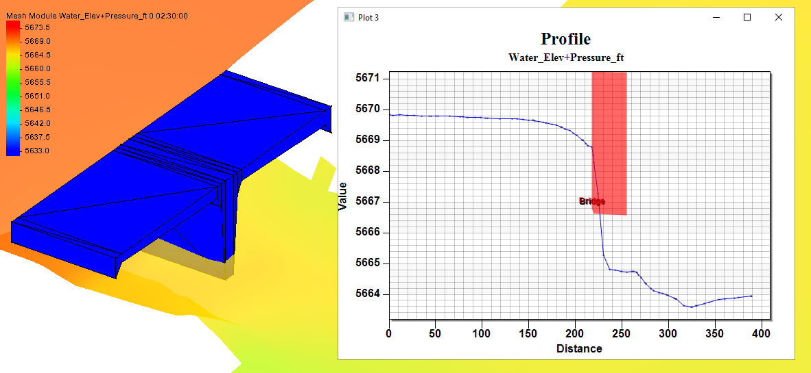
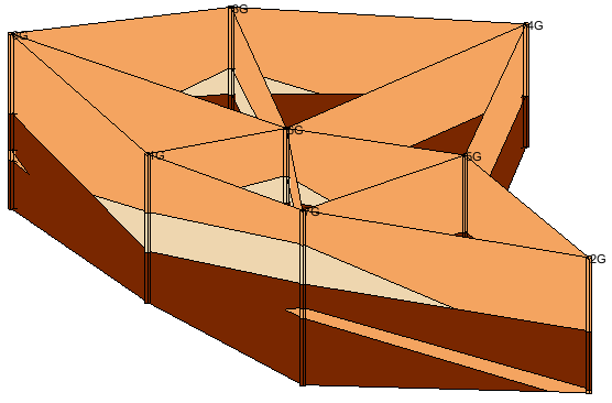
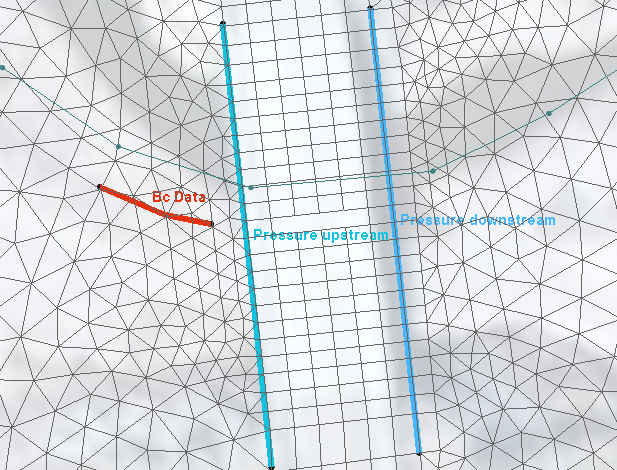
The BCDATA line is primarily used to adjust how flow is calculated going into or leaving a structure. If there is high skew or rapid drawdown at the entry or exit of the structure then you should consider using a BC Data line. It indicates that rather than performing flow computations directly at the site of the structure, they should be performed at the location of the BCDATA line.

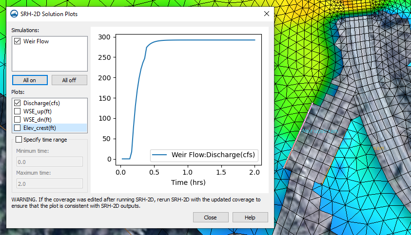
There are a few applications for a BCDATA line. For instance, it can be used on a structure such as a weir or culvert. When SRH-2D computes flow through or over a structure, it uses an average water surface elevation. When no BCDATA line is present, SRH-2D computes right along the nodes where the upstream boundary condition arc has been mapped. If an upstream or downstream BCDATA line exists, the water level can be computed there rather than at the actual edges of the structure. The BCDATA line should typically be located one or two cells upstream or downstream from the structure to get out of the zone of influence of the structure itself. This avoids drawdown caused by the flow going through or over the structure.

To create a BCDATA line and assign it to a structure, use the following workflow:

  1. Use the Create Feature Arc tool to create a line a few elements long, ideally about 1 to 2 elements away from the upstream or downstream arc. Create it perpendicular to the arc and along the centerline.
  2. Using the Select Feature Arc tool, select the line you have just created, right-click it, and select Assign BC… to bring up the SRH2D Assign BC dialog.
  3. Set the BC Type to Bc Data. Make sure to provide a label name that is unique in the coverage. Then click OK to close the dialog.
  4. Now select the upstream or downstream arc that is meant to be associated with the BCDATA line, right-click it, and select Assign BC… to bring up the SRH2D Assign BC dialog.
  5. Scroll down to the General structure options section at the bottom. Depending on whether the arc selected is upstream or downstream, check the box by the appropriate BCDATA line option.
  6. Use the drop-down that populates to select the label you previously specified for the BCDATA line. Then click OK to close the dialog.

The BCDATA line will now be assigned to the structure.

Example of a BCDATA Line

It can also be used on a Link or an EXIT-H boundary condition that you have specified using a rating curve. Normally, without a BCDATA line, SRH-2D computes the average flow directly at the line and then extracts the water level from the curve. When a BCDATA line does exist, the flow rate (Q) is computed across the BCDATA line, like a monitor line, rather than exactly at the boundaries.

Try using BCDATA lines with SRH-2D in SMS 13.1 today!

Blog tags: 

Using A Well Pumping Rate to Calibrate a Model

Have you needed to know how to use a well pumping rate as a calibration parameter in a PEST run? For example, this might be useful in estimating a probabilistic capture zone. We have a workflow that can help with this, utilizing an extraction well and the WEL package for model calibration. This post will review how you can set your MODFLOW parameters in GMS to incorporate well information to be used for parameter estimation.

To do so, use the following steps:

  1. In a well coverage, create a well and give it a constant pumping rate (negative for extraction).
  2. Go to MODFLOW | Parameters... to bring up the Parameters dialog and click the New button to create a new parameter.
  3. Turn on the Show all columns checkbox at the top of the dialog and change the Type value to WELL.
  4. Enter the value that was used for step 1 as the Key, and enter its inverse as the Value.
  5. Enter values for Min and Max that are greater than 0.0. These values and Value will be multiplied by the Q factor later on, which will be -1.0, so positive values listed here will actually become negative.
  6. Turn on the Log Xform checkbox and close the dialog.
  7. Go to MODFLOW | Optional Packages | WEL - Well… to bring up the MODFLOW Well Package dialog.
  8. Enter a Q factor of -1.0 and close the dialog.
  9. Go to MODFLOW | Global Options… to bring up the MODFLOW Global/Basic Package dialog.
  10. Under the Run options section, select Parameter Estimation and close the dialog.
  11. Create a new Observed Flow coverage with Observation Points set to Head in the Coverage Setup dialog, and create a head observation with the Map module active.
  12. Save the project and then click Run MODFLOW to run the PEST Parameter Estimation. When the run is complete, make sure to read the solution into your GMS project.
Example of PEST running using pumping rate as a parameter

Following the above steps will generate solution data where you can use any of the post-processing tools in GMS to review and adjust your model. Try out using well pumping rates in model calibration in GMS 10.5 today!

Blog tags: 

Using a Shapefile with the Fast Flood Tool

Do you have a shapefile with water surface elevation data you would like to use towards quickly generating floodplain data? WMS can help you with this. The Map Flood tool, sometimes called the Fast Flood tool, has a new feature we have developed that will allow you to use shapefiles as part of the process of generating floodplain data. This post will review how to use shapefiles for fast flood mapping in WMS.

Using a shapefile with the Map Flood tool can be done by using the following workflow:

  1. Use any of the methods to open files to import your shapefiles into your WMS project. If your shapefile coordinates are geographic, WMS may ask you to convert them to a planimetric coordinate system for computational use, in which case, click OK to accept this.
  2. The shapefile should now be visible under GIS Data. Click on the Map Flood macro to open the Floodplain Mapping Options dialog.
  3. Under the Water Surface Elevations section of the dialog, click on Use FEMA Floodplain Boundary and select your shapefile from its associated drop-down and after making any other changes, click OK to close the dialog.
  4. Example of using a shapefile with the Map Flood tool
  5. The Virtual Earth Map Locator may appear if there is not a set projection. Use it to navigate to the location of your shapefile then click OK after making any other changes. Navigation can either be done by inputting latitude and longitude or typing in the location you wish to observe.
  6. A message may appear saying that the feature requires a global projection. Click OK on this to bring up the Display Projection dialog.
  7. Review the projection to make certain it is correct, click OK to close the Display Projection dialog and run the floodplain delineation.
  8. After the Map Flood tool finishes, you will have all the necessary data downloaded, and the floodplain will have been generated.

Importing a shapefile into the project will have allowed it to be used with the Map Flood tool instead of needing to download the shapefile. This can save you time and provide consistency when generating multiple floodplains using the Map Flood tool. This also allows you to use a shapefile generated from the first use of Map Flood tool for additional floodplain generation in the same area.

Try out using shapefiles for fast flood mapping in WMS 11.1 today!

Blog tags: 

Viewing a 3D Bridge in a Plot

Have you had difficulty determining where in your plots your 3D bridges are located? At times it can be challenging to determine where objects lie along a generated line plot. This is why SMS has the functionality to be able to tell the plot to display the location of a 3D Bridge. This post will review how to view the location of a 3D bridge in a plot.

3D bridge plot example

The Plot Data coverage provides the ability to locate structures on a profile plot, which could be used to map the location of a 3D Bridge. However, SMS also allows using the Bridge coverage to help see where the 3D bridge is located on the profile plot. It is important to note that a 3D bridge defined within a 3D Bridge coverage will have to be used, as a UGrid will not suffice.

Once you have all your 3D bridges created and defined, you will need to make a profile plot. This is done by using an observation arc within an Observation coverage that intersects the 3D bridge so that it will eventually be visible in the plot. Select that observation arc, and then right-clicking the arc, you must select the Show Observation Plot command to open a Plot window. This plot will automatically update based on which of the datasets and time steps are selected. This plot shows the data values along the observation arc, but by default does not show where a 3D bridge or other structures intersect with the observation arc.

After the profile plot has been generated, right-click within the Plot window and select the Plot Data command to bring up the Data Options dialog. Notice the options in the Components section related to the 3D bridge coverage. Turn on the check boxes for the 3D bridge coverage in any of the relevant rows.

When everything has been set up correctly, the plot will have properly updated itself and you will be able to see a representation of the selected 3D bridges within the Plot window at this point. Now you will be able to properly keep track of where your 3D bridges come into contact with your profile plots.

Try out viewing 3D bridges in a plot in SMS 13.1 today!

Mapping Multiple Coverages in GMS

Do you have a conceptual model project in GMS where you have multiple map coverages with values for the same MODFLOW package? Are you wondering how GMS maps values from multiple coverages over to the MODFLOW packages?

It's not unusual for some projects to require the same attributes to be in separate coverages rather than having all the attributes in a single coverage. For example you might want to use recharge attributes from different sources and have placed the values on different coverages. But how exactly does GMS handle this? This post should hopefully give you a better sense of what GMS is doing behind the scenes.

Normally, the values for a particular MODFLOW package, such as recharge, are placed on one coverage that uses multiple polygons. In this case, a single value can be calculated, taken only from the predominant polygon, as it is expected that the polygons will all be within the same coverage. Also in this case, the methodology is designed to accommodate polygons being used to calibrate recharge zones in PEST, as opposed to calibrating with pilot points. If using gradient recharges, it is recommended to use scatter points to interpolate recharge values to MODFLOW layers.

You may have a case where you have the values for a package, such as recharge, on polygons on different map coverages. This could be because you imported the values from different sources. In cases where the polygons on different map coverage overlap, the attribute types with different values will have those values summed up when they are applied all at once if you map all of the coverages at the same time. If you don’t want them summed up, make sure that rather than applying them all at once, the value you want is the last value mapped over. This is because when multiple coverages are applied at once, GMS sum the values cumulatively, but when done individually, GMS overwrites the value with the most recently mapped coverage.

Mapping multiple coverages

It is important to note that hydraulic conductivity is not cumulative, though the sources may be. Hydraulic conductivity is overwritten every time, so the values MODFLOW receives are the values of the last polygon that intersected an individual cell.

Items in the Project Explorer are mapped in descending order, so changing the order of the coverages can change the end results.

You can also find more information on how objects are mapped to MODFLOW at the Aquaveo XMS Wiki.

Try mapping multiple coverages in GMS 10.5 today!

Blog tags: 

Viewing Multiple GSSHA Scenarios in a Hydrograph

Have you needed to compare multiple GSSHA scenarios using a single hydrograph? New functionality has been added to WMS that now allows for hydrographs that can display results from multiple GSSHA scenarios. This post will review how multiple GSSHA scenarios can be added to hydrographs, a feature newly introduced in WMS 11.1.

Hydrograph showing multiple GSSHA scenarios

Hydrographs that show multiple GSSHA scenarios plot them all out within the same hydrograph. A legend below the graph will indicate which GSSHA scenario run is which in the hydrograph, as each run should be in a different color and potentially a different line style. The dimensions of the hydrograph will be such that all of the different runs will all be able to be displayed.

To be able to work with hydrographs that show multiple GSSHA scenarios, multiple GSSHA scenarios will need to be loaded into WMS to be compared with each other. This can be done by loading multiple GSSHA projects that use the same area into WMS. These can be saved together as a single GSSHA Group Project (GGP) file if needed.

When these GSSHA scenarios will be run, rather than using the typical Run GSSHA command, instead go to the GSSHA | Run GSSHA Group Command. This will open up the Save and Run GSSHA Group dialog. Here, the projects that will run can be selected, as well as the group filename. When the projects have been selected, clicking OK will close out the dialog and bring up the Model Wrapper dialog. This will be brought up for every scenario that will be run, along with the necessary loading of the data into WMS. This will likely take some time, depending on the nature of the GSSHA scenarios, the amount of data to be loaded in, and the amount of different scenarios that will all need to be run.

Once the entire group of GSSHA scenarios has been run, selecting the hydrograph for viewing should display plots of all of the relevant hydrograph scenarios that have been run. Feel free to examine the data, and potentially experiment with different combinations of geographically related runs.

Try out multiple scenario hydrographs in WMS 11.1 today!

Blog tags: 

Using SRH-2D Monitor Plots and Structure Plots

With the release of SMS 13.1, we have added the ability to generate monitor plots and structure plots from the solution of a successful SRH-2D model run. This post will offer a brief rundown of these new features and a brief explanation of how to use them.

SMS now has the ability to generate solution plots at monitoring locations or structure locations, using solution datasets generated during the model run. If you make any edits to the coverage after running SRH-2D, make sure to rerun SRH-2D with the updated coverage to keep the plots consistent with the SRH-2D outputs.

For both plots, they will be displayed in an SRH-2D Solution Plots dialog, and they will have similar options in both cases. These options include:

  • Simulations: contains a list of all available simulations where the monitor or boundary conditions coverages were included during the simulation run. Select which solution set to use for the plot.
  • Plots: contains a list of all available solution datasets from the model run. Datasets you select will appear in the plot.
  • Specify time range: specify the time range for the plot to display. The possible range will be from 0 to the length of the entire simulation.

To use the monitor plots:

  1. Make sure you are in the monitor coverage and select a monitoring point or line.
  2. Right-click to select the Monitor Points Plot or Monitor Lines plot command.

This will open the SRH-2D Solution Plots dialog. Note, you need to make sure the monitor coverage was included in the simulation run, and that only one point or line is selected.

To use the structure plots:

  1. Make sure you are in the boundary conditions coverage and select a structure arc.
  2. Right-click to select the Structure Output Plots command.

This will open the SRH-2D Solution Plots dialog. Note that you need to make sure the boundary conditions coverage was included in the simulation run, and that only one structure arc is selected, even for structures that require two arcs.

Structure plot example

Try using monitor plots and structure plots in SMS 13.1 today!

Blog tags: 

Converting External 3D Materials to 3D Grid Materials

For your 3D grid project in GMS, do you have material data from a 3D mesh or other geometry that was created in an application other than GMS? It is possible to import this data into GMS and attach it to your 3D grid using a method which involves creating solids that GMS can use to assign materials. This is done by importing the data as boreholes and creating solids from them. This post will review how you can take the material data from a 3D mesh and transfer it to a 3D grid in GMS.

To do so, do the following steps:

  1. First, you will need to import the material data as Borehole data into GMS.
  2. You will then need to create horizons for these boreholes. Go to Boreholes | Auto-Assign Horizons.
  3. In the Auto-Assign Horizons dialog, choose Start from scratch, then click Run. The Horizon Optimizer dialog will appear. This step will take a while to complete.
  4. When complete, click "Read solution on exit" and click OK to close out of the dialog.
  5. Once the Horizons are defined, click Boreholes | Auto-Create Blank Cross Sections.
  6. Once blank cross sections exist, click Boreholes | Auto-Fill Blank Cross Sections.
  7. In the Auto-Fill Blank Cross Sections dialog, select what should be matched from the auto-fill options based on the needs of the project.
  8. Cross sections created from borehole data
  9. Create a new coverage, just using the defaults should be fine in most cases.
  10. Using the Plan View and the Create Arc tool, create a closed arc surrounding all of the boreholes.
  11. Select Feature Objects | Build Polygons, to turn this closed arc into a polygon. You might also want to use the Redistribute Vertices command on the arc if needed.
  12. Turn this polygon into a TIN by using Feature Objects | Map → TIN to define the desired boundary of the solid.
  13. Finally, create solids from the boreholes by selecting Boreholes | Horizons → Solids. This will bring up the Horizons to Solids dialog where you can choose your desired settings.
  14. The solids can then be used to classify the materials zone in place of the mesh.
  15. If the solids are needed in another project, you can highlight one or more of the solids in the Project Explorer, right-click, and Export them as a *.sol file.

Try out using this workflow to add data to your projects in GMS 10.5 today!

Blog tags: 

How to Troubleshoot Graphics Card Issues and Display Issues

Out of all the potential issues that can come up, display issues can be some of the most annoying. Display issues can come from individualized hardware configurations, display settings, operating system and software versions which makes solving these issues not as simple as a one-size-fits-all approach. This post will review general best practices for troubleshooting these kinds of issues with your graphics card or display.

Some of the most common display issues that can arise with XMS are problems with one or more of the following:

  • Transparency
  • Functional surface
  • Texture mapping
  • Film loops
  • Contours

The causes behind display issues can be divided into the following categories:

  1. Issue related to remote desktop or virtual machine
  2. Integrated graphics used instead of discrete graphics
  3. Bug in graphics drivers
  4. Limitation of integrated graphics
  5. Bug in XMS affecting all hardware configurations
  6. Bug in XMS affecting specific hardware configurations

Since hardware configurations vary and operating systems change over time, the information here is a general workflow used for troubleshooting.

  1. Remote and Virtual Machine issues: Check if XMS is being run locally or if a virtual machine/remote desktop is being used to rule out Category A.
  2. Versioning: Go to Help | About to note the XMS version, build date, and graphics library used.
  3. Try to rule out Categories E and F: Run XMS in Software Graphics Mode. If the issue is resolved in Software Graphics Mode, then the issue is related to Categories B - D.
  4. Try to rule out Category B: Go to the Device Manager for the Display Adapter. If the driver information/version for the discrete graphics matches what is shown in Help | About, then XMS is using discrete graphics. If not, go to Step 6 to ensure XMS is using discrete graphics.
  5. Device manager
  6. Update graphics drivers: Whether or not the system has discrete graphics, updating the graphics driver will solve some display problems. If the machine already has nVidia or AMD software installed, drivers can be updated through those programs. Otherwise, click the “Update Driver” button (shown in the dialog in Step 4) or Google “GraphicsCard Driver Download” using the graphics card model you have in place of GraphicsCard. Exercise caution with the links you click on. Be sure to click on official AMD, nVidia, or computer manufacturer websites. Avoid 3rd party utilities that offer to optimize your system or install adware/spyware.
  7. Set system to use discrete graphics: Change settings to ensure XMS always utilizes discrete graphics. Many systems, especially laptops, default to power saving modes where programs utilize integrated graphics even if the machine has discrete graphics. The way to change these settings varies by machine.
  8. Reporting Bugs: If Categories A - D have been ruled out, determine if the issue is machine-specific. If reproducible, report to tech support.

If you continue to experience display issues, contact Aquaveo's technical support team.

Blog tags: 

How to Rebuild a Corrupted Project in SMS

Try as we might, we can’t always make everything go according to plan, and sometimes that can include files failing on us. Occasionally, files used in SMS become corrupted and can no longer function properly.

This can happen for a few reasons. A file may have been blocked from saving correctly by the computer’s system security. The save process may have terminated early. The project files may have been copied incorrectly. The project files may have been stored incorrectly. Or some other unknown error may have occurred.

Project load error

While the corrupted project file itself cannot be restored, the component pieces of the project can be reassembled in SMS and saved out as part of a new project file. Below is a list of the file types you will need to reassemble:

  • [project name].map: These are the Map Module coverages saved to the project. The model-specific boundary conditions will likely need to be entered again.
  • [project name]_meshes.h5: These are the meshes that were in the project for models that use a mesh. Load this before loading any of the datasets saved in the [project name]_datasets folder.
  • [project name]_grds.h5: These are the grids that were in the project for models that use a grid. Load this before loading any of the datasets saved in the [project name]_datasets folder.
  • [project name].h5: This contains scatter sets that were in the project.
  • Any GIS layers, such as rasters or shapefiles, will also need to be loaded again.

For ADCIRC models, use the following files to import the ADCIRC simulations:

  • Use the fort.14 or fort.15 files to import the mesh and create the simulation.
  • Also import solution files such as fort.63, fort.64, maxele.63, and maxvel.63 files.

For CMS-Flow, use the following files to import the CMS-Flow simulations:

  • Use the [project name].cmcards file to import the UGrid and create the CMS-Flow simulation.
  • To load solutions for the CMS-Flow simulation, import the [project name].h5 files.

For SRH-2D models, use the following files to import the SRH-2D simulations:

  • Reload SRH-2D simulations (including the coverages linked to them) by loading the SRHHYDRO file, found under the [project name]\SRH-2D\[simulation name] folder.
  • To load solutions for SRH-2D simulations that were already run, import the XMDF.h5 file from the same directory as the SRHHYDRO file.

For STWAVE models, use the following files to import the SRH-2D simulations:

  • Reload STWAVE simulations (including the coverages linked to them) by loading the [simulation name].sim file, found under the simulation folder.

It is strongly recommended that a thorough review of the project should be completed before you continue working with the rebuilt project.

When your files become corrupted, please contact Aquaveo Technical Support (support@aquaveo.com) to report the issue.

If you have issues with corrupted projects in SMS, try following some of these steps to fix them in SMS 13.1 today!

Blog tags: 

Pages