Aquaveo & Water Resources Engineering News

How to Calculate Riprap Using the Hydraulic Toolbox

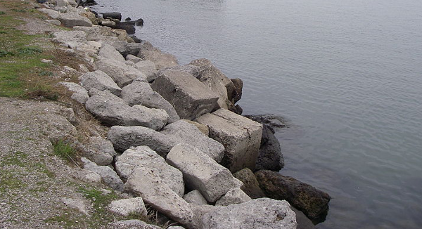
Are you needing to determine the size of stones needed for riprap? Having stones that are too small will reduce the effectiveness of the riprap which could be disastrous. On the other side, having stones that are too large could cause unnecessary expense.

After defining drainage data in WMS, it is possible to calculate the riprap needed for your model using the FHWA Hydraulic Toolbox. To do this:

  1. Define your drainage data in WMS.
  2. Assign each basin attribute to an analysis method by double-clicking on the feature, and then selecting Edit Attributes…. This will give you the opportunity to link your drainage data to the Hydraulic Toolbox.
  3. Click on the Hydraulic Toolbox macro in WMS to bring up the Hydraulic Toolbox.
  4. You can calculate riprap using one of two methods:
    • Channel Lining Design Analysis Tool. Keep in mind when using this tool that a filter material must be separately designed.
    • Riprap Analysis Tool. This tool will calculate the filter material along with riprap size.

Once in the Hydraulic Toolbox, locate the name of the analysis method chosen and double-click to open the analysis dialog for the chosen parameter and method. You will notice that all of the data you input into WMS is now filled in the analysis tool. After you specify blank parameters, the tool will calculate and display the results at the bottom of the screen under “Minimum Riprap Thickness”.

Using the Hydraulic Toolbox to calculate riprap can help your project move forward. The toolbox also contains many other features worth exploring. Try using the Hydraulic Toolbox today!
Blog tags: 

Aquaveo Visits Namibia

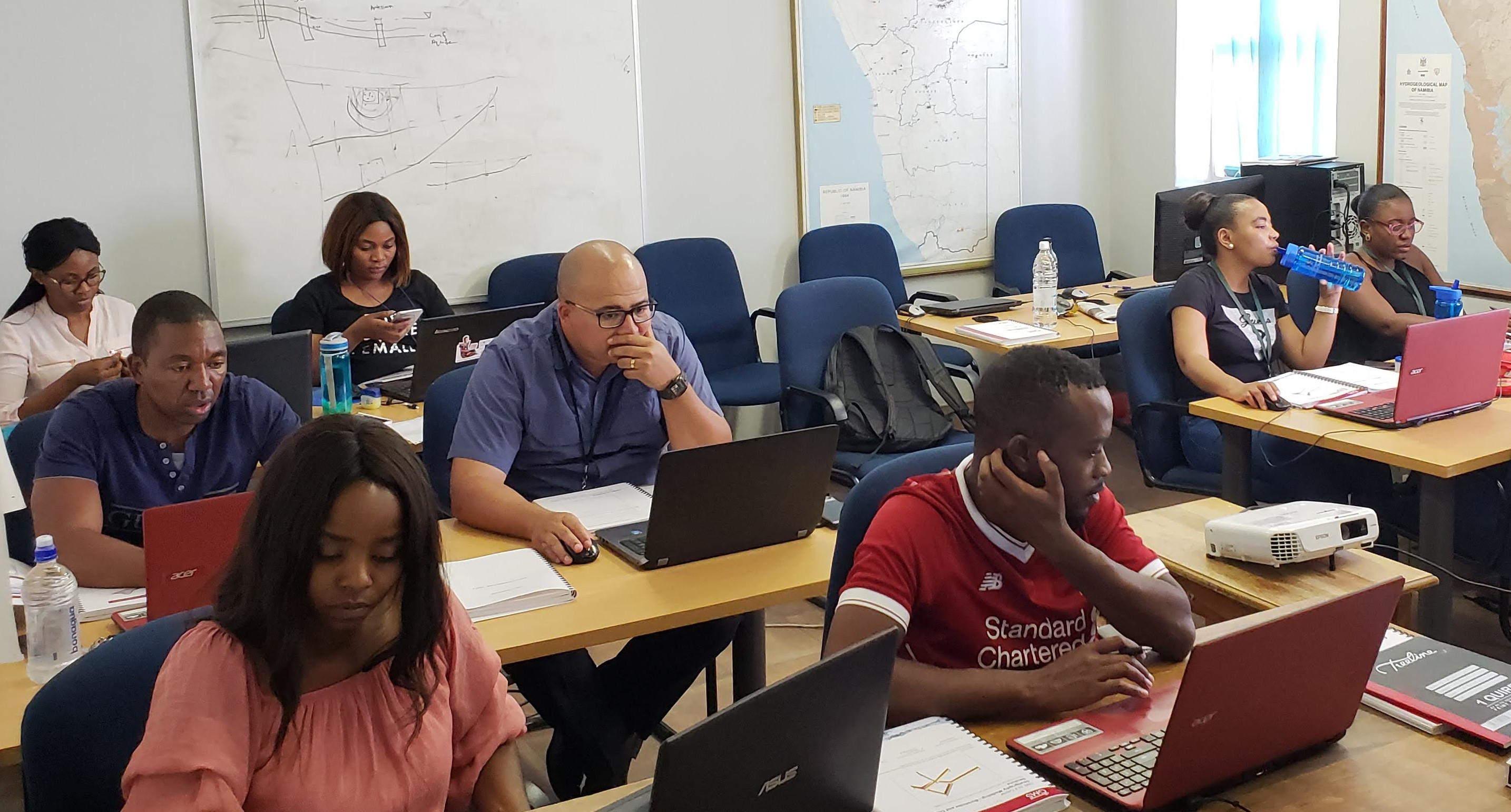
From November 6-9, Aquaveo had the privilege of traveling to Windhoek, Namibia to conduct a training and provide consulting sponsored by BGR for several employees of MWAF. The Ministry graciously provided space in its building for the training classes. During the training classes, Alan Lemon helped them refine a MODFLOW model of the Ohangwena II aquifer.

Northern Namibia has a long history of droughts, and Namibia is the driest country in sub-Saharan Africa. Surface water is not a reliable source for potable water in the area due to the infrequency of rain storms to replenish the watershed. Because of this, the Namibian government—through its Ministry of Agriculture, Water, and Forestry (MWAF)—partnered in 2012 with the German Federal Institute for Geosciences and Natural Resources (Bundesanstalt für Geowissenschaften und Rohstoffe, or BGR) to research and develop an aquifer discovered near the northern border with Angola.

The Ohangwena II aquifer is found below an area about 75 km by 40 km, and has nearly 20 billion cubic meters of fresh water. This is enough to last for well over 400 years at current usage levels, and some think there may be even more water there. This kind of resource would be invaluable to the Namibian people.

Creating a valid working model of the aquifer will help the government of Namibia and BGR to come up with a solid groundwater management plan. Such a plan will help them better manage this amazing resource so that the people living in northern Namibia will have the water they need while also preventing needless wasting of hundreds of years of water located in the precious aquifer.

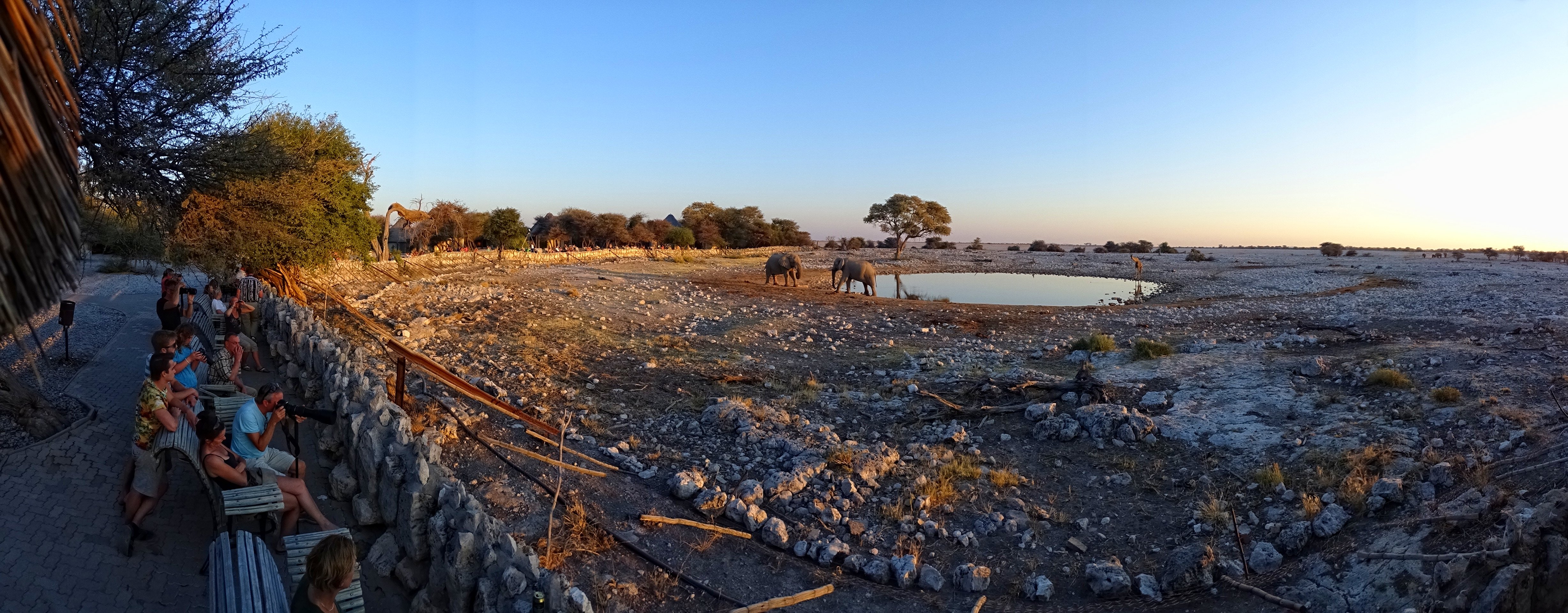
During the trip, Alan had the chance to visit the Okaukuejo Waterhole in Etosha National Park, where he saw a number of different animals, including rhinoceroses, crocodiles, and springbok. The watering hole is visited by tens of thousands of animals each year, from small birds and mammals to some of the largest and most dangerous animals in Africa. The national park is near the area covered by the Ohangwena II aquifer.

We want to thank BGR and MAWF for inviting us to their facility, and for the opportunity to work on such an important project. If you are interested in having Aquaveo assist with your projects, check out our consulting services.

Blog tags: 

New Floodway Delineation Tool in SMS 13.0

City planners, developers, and others have a great interest in using available land. Sometimes that land is close to areas that flood, so precautions need to be taken so the build site is not too close to (or directly in) the potential flood area. Failure to properly plan and delineate a floodway can potentially cause millions of dollars in flood damage as well as potential losses in property values. Hurricanes Harvey and Florence, with their extreme rainfall amounts, are prime example of why floodway delineation is so important.

In addition to the guidance provided by the Federal Emergency Management Agency (FEMA), the new Floodway tool in SMS allows the extents of a floodway area to be more clearly defined. This tool allows planners, developers, and others to run multiple simulations to determine the safest places to build as well as the places which may be most impacted during a significant flooding incident.

To use the Floodway tool in SMS, a project must have a either a Cartesian grid, a 2D mesh, or a 2D scatter set that has simulation result datasets for at least water depth and velocity. Two coverages are also required: a 1D hydraulic centerline coverage and a 1D hydraulic cross section coverage.

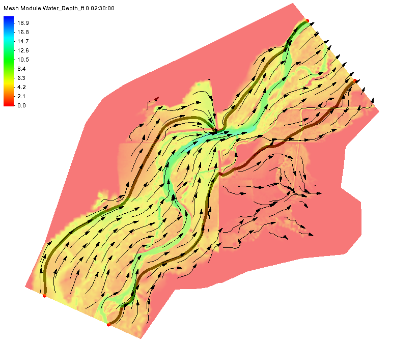
The way the Floodway tool works is by calculating how far in from both sides of a river or stream that vertical walls can be placed and raise the center of flow by the targeted maximum rise. FEMA suggests this rise should be no more than 1 foot. These calculations use the input provided by the water depth dataset, the velocity dataset, and the two hydraulic coverages to define the floodway extents along the entire length of the study area.

Once these extents are known, the data can be used when making area planning and development decisions at all levels of government and businesses. You can try out this feature in SMS 13.0 beta today.

Blog tags: 

New and Improved Lidar Tools in GMS 10.4

With the release of GMS 10.4 (beta), a set of new and improved tools for importing and handling lidar files is now available. The new tools provide much faster import times, and most processing happens on the fly as the lidar display options are adjusted.

Merging and Display Options

As with previous versions of GMS, either a single or multiple lidar files can be imported. However, the options available for handling the lidar data have changed significantly, offering more precise control and more options that will allow better use of the lidar file data.

One of the best new features is that GMS 10.4 allows merging multiple lidar files into a single file. This is accomplished by selecting the desired lidar files in the Project Explorer, then right-clicking and selecting Merge. Enter the desired filename and allow GMS to process the merge.

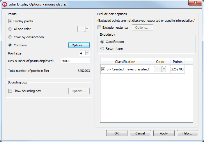
After the merging is complete, you can import the new lidar file into your project.The merged file has all of the lidar cloud points that were contained in the original lidar files, though not all of them may be visible. The visibility of lidar cloud points can be adjusted using the display options for the merged lidar file. Access them by right-clicking on the merged lidar file in the Project Explorer and selecting Display Options… to bring up the Display Options dialog.

]

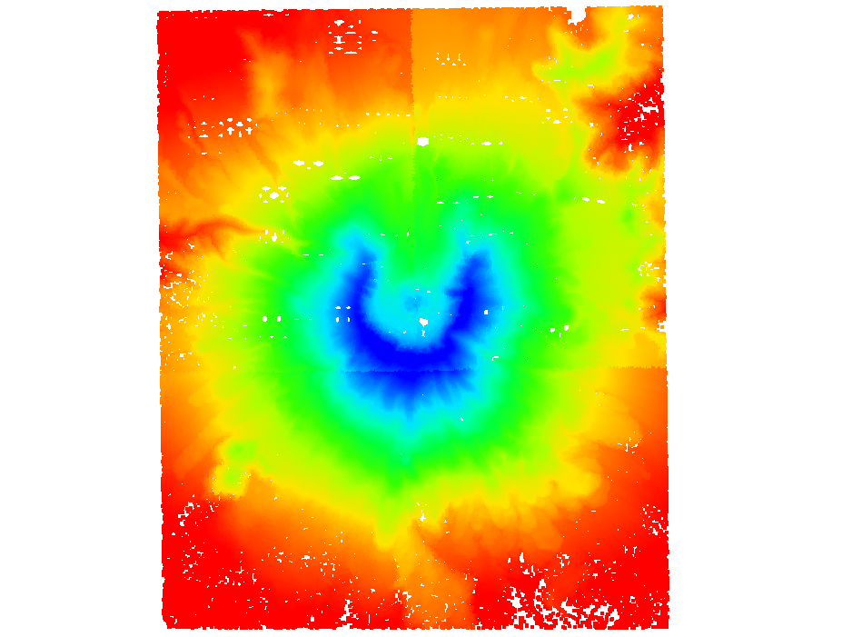
This dialog allows you to change point size, how many are displayed, which kinds are displayed, which points to exclude, and how to exclude them. This allows you to choose the level of complexity without overwhelming you with too many options. The following image shows the merged lidar file with 5 million points displayed.

Interpolation Options

  • UGrid: If your project has an existing unstructured grid (or one that has been imported or created), you can interpolate the lidar files to that UGrid. Simply select the desired lidar files in the Project Explorer, then right-click on them and select Interpolate to UGrid… to bring up the Interpolate Lidar to UGrid dialog. This allows you to select the target UGrid, set the new dataset name, and set the sampling distance.
  • Raster: This option uses the lidar display options set at the time of interpolation and creates a raster file. The Interpolate Lidar to Raster dialog allows the number of X and Y cells to be set, and changing those affects the cell size. The merged raster is then imported into the Project Explorer.

Try these new features today in GMS 10.4 (beta).

Blog tags: