Aquaveo & Water Resources Engineering News

Using the Prune Arc Tool

The Prune Arc tool is relatively new to SMS, and we're excited to show you just how useful it can be.

The Prune Arc tool is similar to the smooth arc function in SMS. This Smooth Arc tool is useful when eliminating noise from a rough arc, and can make your variations more mathematically stable. This can be extremely handy in working with a model—especially in situations like coastal modelling, which are prone to busy edges. Unfortunately, smoothing an arc can also change the shape of the arc to the point where it no longer matches the actual coastline.

You may come across a situation where your imported arcs have a lot of unnecessary roughness or concave areas that you want to eliminate without redistributing your vertices along the rest of the arc.

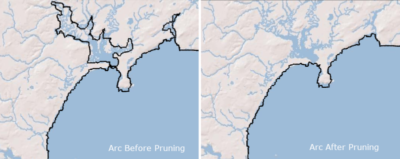
If this is the case, the Prune Arcs function is just the tool for the job. This tool trims—or prunes—rough edges and outlying spikes without rounding or reshaping the rest of the arc. Specifically, it allows you to focus on smoothing one side of the arc. This is helpful in coastal modeling where there may be a small river mouth, a harbor, cove or other concave sections that you do not want to include in your model.

Prune arc example

Access the Prune Arc tool by doing the following:

  1. Use the Select Feature Arcs tool to choose the arc or arcs you wish to prune.
  2. Right-click on the selected arcs then, in the menu, select the Prune Arc(s) command.

This will bring up the Prune Arcs dialog box, from which you can choose your pruning settings.

There are two types of pruning that can be done: Constant and Spatially Varying.

  • Constant will prune everything within a specific measurement set by you. This measurement is in meters by default. The larger the number, the more dramatic the pruning will be.
  • Spatially Varying uses the numbers in a particular dataset to establish the parameters of the pruning. This dataset is chosen in the Prune Arcs dialog box.

Importantly, you must choose which side of the arc to prune. The sides of the arc are determined by the arc direction. So if the arc is moving south to north, the left side of the arc will be on the left side of your screen. If the arc is moving west to east, the left side with be towards the top of your screen. Make certain you are pruning the correct side of the arc.

Try out using the Prune Arc tool in SMS 13.0 today!

Blog tags: 

Tips for Using Multiple Conceptual Models

Have you ever built a model in GMS that uses multiple conceptual models? Doing this offers a few advantages. However, there are potential pitfalls as well when doing this. We will discuss some of the advantages in using multiple conceptual models and what to watch out for.

A conceptual model may contain one or more map coverages. Each coverage should contain feature objects defining key structures of the groundwater model, such as wells, rivers, or recharge. Everything in the conceptual model can then be mapped over to a grid or MODFLOW model.

Example of multiple conceptual models in the Project Explorer

Beyond using folders under a single conceptual model, one of the main advantages with using multiple conceptual models is for organization. When wanting to make variations on a model, it is helpful to have one base conceptual model and then multiple variant conceptual models. The entire base conceptual model may be duplicated to provide a starting point for other variations, or individual coverages may be duplicated and dragged to other conceptual models. Duplicating the base conceptual model can be particularly helpful if you already have transport species defined for MODFLOW-related models.

For example, you can use one conceptual model for a base steady-state model, then create another conceptual model for a transient predictive model. With this you can map the base conceptual model to MODFLOW and run that model. After you have the base results, you can duplicate the solution datasets to preserve them, adjust Global Options—such as Stress Periods—if needed, and then map the predictive model to the grid to run your second MODFLOW model.

When using multiple conceptual models, there are few items to look out for. These include:

  • When changing the conceptual model, changes are not automatically made to the MODFLOW model or other models being used. The conceptual model must be mapped over to the groundwater model in order for the defined features to be included in the model run.
  • When mapping over the conceptual model, it will overwrite any existing data in the same packages contained in the conceptual model. If you want to update the model with the new conceptual model, this is the correct workflow. However, if the original conceptual model used packages that are no longer used in the new conceptual model, then there could be an error in the model run. Always review your model after mapping to confirm the features mapped as you intended.
  • When using MODFLOW-USG, and you have multiple UGrids, make certain the conceptual model is mapping to the correct UGrid or model. It will map to the active UGrid.

Working with multiple conceptual models can expand your options for your model. Try out the conceptual model and other features of GMS today!

Blog tags: 

Converting a 2D Scatter to a Raster

Have you ever needed to convert a 2D scatter set to a raster? A new feature of SMS 13.0 allows converting a 2D scatter set to a raster from the right-click menu in the Project Explorer.

Being able to convert from a 2D scatter set to a raster is particularly useful when collaborating with a colleague, or switching between programs. There are many types of raster files that can be shared between different applications.

To convert a 2D Scatter right-click on the 2D Scatter Set under Scatter Data folder in the Project Explorer and go to Convert | Scatter → Raster.

In the Interpolate to Raster dialog you have three options for Interpolation:

  • Linear
  • Inverse Distance Weighted
  • Natural Neighbor

Each option for interpolation is slightly different from the other focusing more on lower z values, higher z values, or the x and y values. Feel free to compare all three with your 2D scatter set.

Once you have selected the interpolation type you can choose to truncate some of the data by clicking on the Options button to launch the Interpolate dialog. Using the truncating option removes data from your raster. Some scenarios many only be visible in Plan view.

When you have selected your interpolation method, and truncation value if you so desire, then selecting OK will direct you to saving your raster file. You have two file type options:

  • Geo TIFF Tiles (*.tif)
  • Arch Info ASCII Grid Files (*.asc)

If you select the ASCII file type you may be asked to select a global projection, whereas the TIFF option does not. By default the raster will be imported into your current project.

When converting a scatter set to a raster the program may need to make some adjustments to outlying points. With each of the interpolation options, SMS adjusts the data for slightly different raster results.

You can see that the converted raster closely reflects the original dataset. The scale on the left of the Graphic Window will show you how closely the two are alike.

2D raster to scatter example

Now that you know how easy it is to convert a 2D scatter set to a raster try it in SMS today!

Blog tags: 

Aquaveo User Conference 2019

The 2019 Aquaveo User Conference is going on now. It started yesterday, October 8th, and will wrap up today, October 9th. We are enjoying meeting with users from around the world. In attendance are users from the United States, Germany, Portugal, South Africa, and other places around the globe.

At the conference, we announced some of the new features and upcoming changes to our products that we are excited about:

  • Making XMS functionality available for use outside of the traditional interface.
  • More web-based applications for portability and ease of access.
  • Simplifying and unifying tools so it is easier to find and use the functionalities available.
  • Project management tools to track the history of a model.
  • 3D bridge modeling in SMS.
2019 Aquaveo User Conference

Talking to those in attendance, we learned they enjoyed:

  • Learning more about software features and functionality.
  • Learning how to improve their model development process.
  • Discovering benefits of Aquaveo’s software over other software.
  • Talking to developers and learning tips for model development.
  • Being able to show off their models and receive feedback on them.
Eva Loch presenting at the 2019 Aquaveo User Conference

We’d like the thank the following for participating during our user conference:

If you couldn’t make it to the Aquaveo User Conference this year, watch our website and Facebook page for future conferences.

Classifying Material Zones

Do you ever struggle to assign materials to a grid from solids? In GMS, the Solids to MODFLOW command is a useful tool for this, but it’s not successful in all cases. This command can sometimes make alterations to the stratigraphy. The command also does not work with models that make use of a mesh.

The good news is, there is another way! The Classify Material Zones command allows you to assign material zones from solids to a grid using just a few steps. The general workflow for doing this is as follows:

  1. First, you'll want to create a grid or mesh that is the same shape and has as many layers as your solids.
  2. Next, right-click on your grid and choose the Classify Material Zones command.
  3. In the Classify Material Zones dialog, ensure that your solids are selected and choose your desired classify algorithm.
  4. Finally, click OK and your grid materials will be matched to the solids.

When setting the classify algorithm, there are two options: "Centroid" and "Predominant material". The "Centroid" option assigns each cell the material located at its centroid. Using the "Predominant material" option assigns each cell the material that is present in the highest volume.

Below is a comparison between the two classify algorithms on a sample grid, "Centroid" on the left and "Predominant material" on the right. Select the algorithm that best represents your modeling area.

Example of the Classify Zones algorithms

The end result of using the Classify Materials Zones tool is that a new material set, based on the materials in your solids, will be added to your grid or mesh.

Try using the Classify Material Zones tool in GMS today!

Blog tags: