Aquaveo & Water Resources Engineering News

New Color Ramp Options for SMS

By aquaveo on August 29, 2023

The contour options in the Surface-water Modeling System have been overhauled and expanded in SMS 13.3. It includes many new color palettes to apply to a selected mesh or grid, making it so you can customize your project more than ever before.

SMS's color palettes are accessed by clicking Color Ramp… on the Contours tab in the Display Options dialog. When you right-click on a color palette in the Choose color ramp dialog, two options appear: "Make favorite" and "Make editable copy". If you select "Make favorite" a new folder will appear at the top of the dialog with your favorites. This is a good option if there is a specific color palette you want to keep track of for use in future projects. If you select "Make editable copy", you’ll see more options in the right-click menu. The new options in the right-click menu for the newly editable color palette are edit, rename, duplicate, and remove from project.

Example of the Choose Color Ramp dialog in SMS 13.3

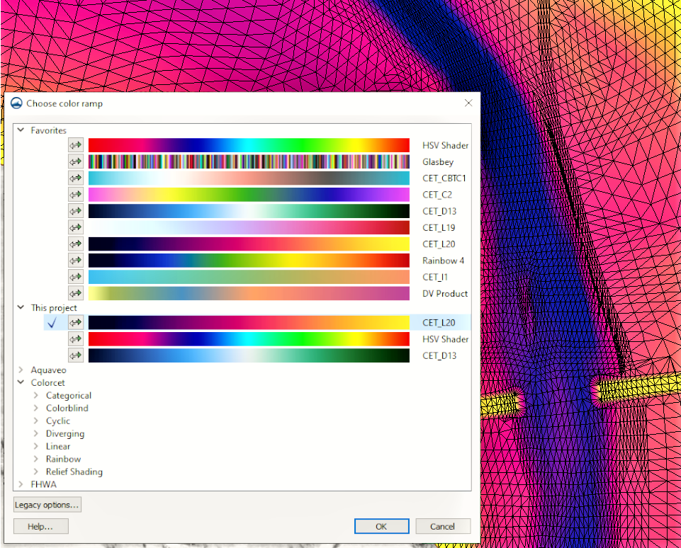
There are five sections on the Choose color ramp dialog:

Favorites: this folder will appear when you designate a color palette as a favorite. This is a great option to keep track of your favorite color palettes, and save any color palettes that you've customized so you don’t lose them if you want to use them later.
This project: includes every color palette selected for use in the current project. SMS allows you to customize the contours of any mesh or grid in the project, or even every mesh or grid, if that is something you want.
Aquaveo: we took note of the palettes that are most commonly used, and we put a pre-generated version of those palettes under the Aquaveo folder so it is easy for you to access.
Colorcet: this includes various additional folders that categorize specific color palettes. These folders consist of:
- Categorical: Contains color palettes where colors are assigned to specific values or categories.
- Colorblind: Contains color palettes designed for individuals with color blindness.
- Cyclic: Contains color palettes optimized for cycling through the colors in a seamless manner.
- Diverging: Contains color palettes that primarily consist of two colors separated by white or black.
- Linear: Contains monochromatic or dual chromatic color palettes.
- Rainbow: Contains color palettes with a full spectrum of colors.
- Relief Shading: Contains color palettes specifically optimized for use with relief shading.
FHWA: contains a list of FHWA specified color palettes. We worked with the Federal Highway Administration to develop specific palettes for use with their two-dimensional hydraulic modeling technologies. The use of these palettes isn't limited to FHWA models, but you should definitely check them out if you’re working with models developed by FHWA on a regular basis.

There is a "Reverse color ramps" button next to every color palette. This button does exactly what it sounds like. It reverses the color gradient so that the color the color palette previously ended with is now the starting color, and vice versa.

A Legacy options… button is in the Choose color ramp dialog, which will take you to the Color Ramp Options dialog that you may be more familiar with from previous versions of SMS. If you're used to the way that the color ramp options used to work and prefer to stick with that, we've got you. This dialog has everything you knew and loved about customizing color ramps from the older versions of SMS, and will work the same way.

There are many color palettes and contour options to explore, download SMS 13.3 and see how they can enhance your project today!

Blog tags:

SMS

Exporting Transient Observation Data

By aquaveo on August 22, 2023

When working with transient data in the Groundwater Modeling System (GMS), having a way to view the generated Plot Wizard. The Plot Wizard is found under the Display menu at the top of the GMS window. The Plot Wizard opens to a dialog containing a list of all the available plot types. If you're not sure which plot type will contain the data you're looking for, a short description of the selected plot will appear on the right under the plot preview.

Once you finish the set up in the Plot Wizard and the plot is generated, you can right-click on the plot window and select "View Values" to bring up the View Values dialog. This dialog contains a simple data table which includes a list of all points and observed points, as well as a list of all time steps and their related value.

Exporting Transient Observation Data from the Plot Wizard

The second method to view observation data is by going to the MODFLOW menu at the top of the window and selecting Observations. This method opens a window which will allow you to export a CSV file that contains all the observation data. Make sure that "Use" is turned on for the Observation Wells coverage, and then click "Export Trans. Obs…" to bring up the Transient Observation Filename dialog. Although the "Save as type" dropdown may indicate that the data can only be exported as a TXT file, it will actually save as a CSV file. The CSV file contains a more comprehensive table of all the observation data than the Plot Wizard does.

CSV Format of Exported Transient Observation Data

The given data for the exported observation data is divided into several groups. Each group contains a list of observation times, the corresponding recorded value, and the computed value at those specific times. This is sometimes different from the output times from the calculated list, so it offers precise values for comparison, removing the need for estimation based on the output list.

Head over to GMS and check out how this can improve how you view transient data today!

Blog tags:

GMS

ASCII Grid Files for GSSHA in WMS

By aquaveo on August 15, 2023

The Watershed Modeling System (WMS) offers powerful tools for managing and analyzing spatial data using ASCII files. In this blog post, we will explore WMS ASCII files, discuss specific file formats like the *.dep (DEPTH) and *.gfl (FLOOD_GRID) outputs as well as the possibility of exporting ASCII gridded files for GSSHA.

WMS utilizes ASCII files to store and exchange spatial data, such as boundaries, elevation data, and model outputs. To extract information from these files, it is helpful to understand their formatting. The WMS ASCII file contains coordinates representing the boundary limits of the data. However, a common question arises regarding whether these coordinates represent the corner or center of the boundary cells. The coordinates provided in a file header can represent the lower left corner of the cells rather than their center. This information is for accurately defining the spatial coverage of the data.

ASCII Gridded Files Format

WMS is capable of outputting files containing spatial information as grid files, such as the DEP and GFL files. These files store multidimensional data (time, x, y) in a single column format. In the DEP and GFL files, as well as other GSSHA files, the data is organized by cell ID. The introductory information in the file provides details such as the type of information, geometry type, number of cells and values, and dataset name. Each time step is indicated by the TS field, followed by the corresponding data. The dataset file concludes with a flag indicating the end of the data.

Exporting ASCII Gridded Files with GSSHA

While discussing GSSHA, it is important to note that it employs cell-centered Cartesian grids. It is also important to note that GSSHA does not offer alternative export formats for gridded files, apart from the ASCII-based output options provided in WMS. These options can be found by doing the following:

Select GSSHA | Job Control command to open the GSSHA Job Control Parameters dialog.
Click the Output Control button to open the GSSHA to Output Options dialog.
In this dialog, make certain that the ASCII option is selected for output.

ASCII gridded files are one of the many options you can use with GSSHA in WMS. Try out ASCII files and other formats in WMS today!

Blog tags:

WMS

Utilizing SMS's Gravity Waves Tools

By aquaveo on August 8, 2023

Are you working with a coastal model in the Surface-water Modeling System (SMS) that includes a representation of how particles move through a mesh or grid? Did you know that the toolbox has Gravity Waves tools, which can help you visualize and find data about those particles more easily? This blog post will give you an overview of both the Gravity Waves Courant Number tool and the Gravity Waves Time Step tool and how they can help you with your ocean models such as ADCIRC.

The Courant number is a value that represents the amount of time a particle stays in the cell of a mesh or grid. The purpose of the Gravity Wave Courant Number tool is to help maintain the stability of a numerical engine and, potentially, to help choose the most suitable time step measurement. If the methods used to solve numerical problems are restricted by the Courant condition, things can become unstable if the Courant number goes beyond the allowed limit. By looking at the highest Courant number in the dataset, you can get an idea of how stable the mesh is with respect to the chosen time step.

There are three necessary input parameters for the Gravity Waves Courant Number tool, the first being a dataset. This tool requires a dataset that represents the particle’s velocity magnitude. Second, you need to enter a gravity value. Lastly, you’ll enter a computational time step value. For the output parameters, you’ll choose a name for the new dataset. It should be something short and easily recognizable, possibly referencing the input dataset.

The Gravity Waves Time Step tool functions as somewhat the opposite of the Gravity Waves Courant Number tool. The purpose of the Gravity Waves Time Step tool is to calculate the time step needed to achieve the desired Courant number, based on the provided mesh and velocity field. You can then choose a time step for analysis that is equal to or greater than the highest value in the resulting dataset of time steps.

The required input parameters for the Gravity Waves Time Step tool are first, an input dataset, which should be set for depth. Note that it is important that the dataset is specifically for depth, not elevation. Second, enter a gravity value. Lastly, enter the Courant number you’re searching for. Choosing a value for the Courant number under the maximum threshold may increase the stability of the computation because the resulting computation is approximate. The output parameters are where you’ll specify a name for the new dataset. As with the Gravity Waves Courant Number tool, the name should be something short and descriptive.

Try out the Gravity Waves tools for yourself, and see what they can do for your SMS project today!

Blog tags:

SMS

Calculate the Water Level Below the Top of an Aquifer

By aquaveo on August 1, 2023

The Data Calculator is a useful feature that is available in the Groundwater Modeling System (GMS). The Data Calculator performs many functions and can enhance your project and simplify the visualization of data. This blog post will provide an overview of how to use the Data Calculator in GMS to pinpoint locations where the water level in a selected aquifer falls below the top elevation in a MODFLOW simulation.

Calculating the Water Level Below the Aquifer

As you might expect, a MODFLOW simulation containing aquifers needs to be completed before you are able to use the Data Calculator to find the time step where the water level falls lower than the top elevation in the simulation. The datasets required for this calculation are the top elevation dataset and the head dataset.

Before opening the Data Calculator, you will first need to duplicate the top elevation dataset. This is because the Data Calculator isn’t able to recognize the datasets directly under the MODFLOW simulation in the Project Explorer. Right-clicking on the top elevation dataset and selecting duplicate will create a copy of the dataset under the grid folder in the Project Explorer, and this duplicate can now be read into the calculator. If desired, you can right-click on the duplicate dataset and rename it to something that makes more sense to you.

The next step is to go to the Edit menu at the top of the screen and select Dataset Calculator to open the Data Calculator dialog. There is also a Data Calculator macro on the top row, which will bring up the same dialog. Follow these general steps to calculate the data once the Data Calculator is open:

On the left side of the dialog, find and select the Head dataset.
On the right side of the dialog, either select a specific time step from the list, or check the box that says “Use all time steps”.
Click the “Add to Expression” button to add the Head data at the selected time steps to the calculation.
Click the subtraction button (-), or use your keyboard to type the subtraction symbol.
Select the copy you made of the top elevation dataset and click “Add to Expression”.
In the Result field, enter a name for the new dataset.
Press Compute, then click done to close the dialog.

After generating the new dataset, you can right-click on it in the Project Explorer and select “View Values”, which will let you view the data values for the selected time step. Any values denoted by a negative number indicate a water level lower than the highest point of the aquifer.

Head over to GMS and see the many ways the Data Calculator feature can be useful to you and your project!

Blog tags:

GMS