Aquaveo & Water Resources Engineering News

Using the Snap Preview Option

Having trouble with your boundary conditions or materials not aligning correctly with your mesh?

When a simulation runs in SMS, it takes all of the components—such as boundary conditions and materials—and aligns them with the 2D mesh or other geometry. When creating boundary conditions in the Map module for SRH-2D, ADCIRC, or other models that use simulation components, it can sometimes be difficult to know exactly where the boundary conditions will line up with the 2D mesh nodes.

To help with this, the boundary conditions map coverage contains a display option to see how the map arcs and mesh nodes will line up: the Snap Preview option.

To use the Snap Preview option, do the following:

  1. Make certain the project contains a 2D mesh and a boundary conditions coverage that have been linked to a model simulation
  2. Open the Display Options dialog
  3. On the Map tab of the dialog, turn on the Snap Preview option

The Snap Preview option can also be turned on or off by using the Shift+Q shortcut key.

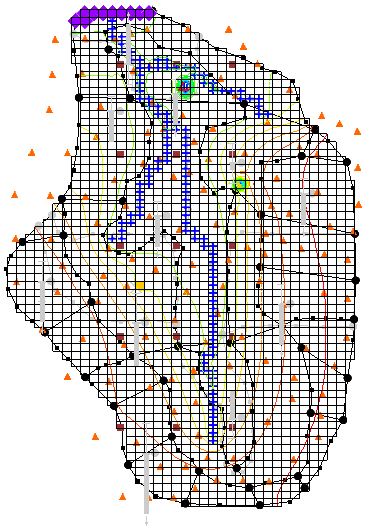
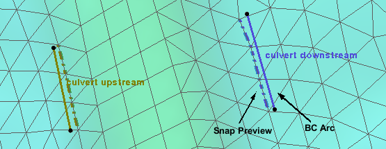
When the Snap Preview option has been turned on, a dashed line will be displayed along the element edge to show where the boundary condition arcs will match up with the mesh nodes. This is helpful in identifying if the placement of the boundary condition arcs is correct. Incorrect placement of boundary condition arcs can cause errors in the model run.

Snap Preview Example

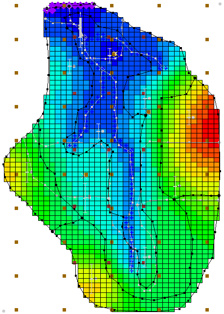
The Snap Preview option also works for other model coverages such as the SRH-2D materials coverage. This allows previewing how material assignments will match up with the mesh elements. Adjustments can then be made to the material polygons to correct any misalignments.

Using the Snap Preview option can significantly reduce frustration and prevent errors early on. Try using Snap Preview in your SMS projects today!

Blog tags: 

Tips for Working with PEST

Parameter estimation using PEST can assist in data interpretation, model calibration, and predictive analysis. PEST can do a lot for your project.

Because PEST offers so much, it can be a little overwhelming to use at first. We provide tutorials and articles on our wiki to help guide you in using PEST with GMS.

In addition to the resources available in the tutorials and wiki, this post covers some useful tips that have helped some of our users.

General PEST Tips
Model calibrated using PEST

Here are some general tips for troubleshooting PEST in GMS:

  • Verify that the parameter key values have been successfully initialized under MODFLOW | Parameters. The key values should match the parameters names. For example, if the key value for hydraulic conductivity is “-30”, the parameter name should be “HK_30”. No key value should be used twice, even across different packages. To continue the example, if you have an “HK_30”, there should not be a “RCH_30”.
  • Key values are needed for both zones and pilot points.
  • Key values are expected to be negative integers. Non-integers will not be automatically recognized as key values.
  • If the key value is not a negative integer, or is a parameter from the WEL package, they will have to be manually added. If you’re missing a value, check that it initialized in the first place.
  • Parameters included in the run will be written to the *.param file. Once PEST runs, the optimal values are written to the *.par file.
  • If the iterations are giving identical values for the same parameter, check if the value is either the minimum or the maximum of the range assigned to the parameter, then evaluate if that range needs adjusting.
  • Adjusting the starting values or the PEST options may help.
Pilot Point Tips
PEST with pilot points

When using PEST and pilot points, consider the following:

  • Follow the recommended guidelines found here.
  • You can get a quick 2D Scatter set to use for pilot points with the MODFLOW Layers → 2D Scatter Points tool. This is particularly useful for areal parameters, such as HK or RCH.
  • If you’re running Null Space Monte Carlo, you must use pilot points and your interpolation method must be set to kriging.
  • If running with SVD-Assist, you can point to the Jacobian file so it doesn’t re-solve for every iteration.
  • Depending on the parameter, pilot points often should not start with zero values. This especially applies to log transforms.

We hope these tips help and that your project are improved by using PEST with GMS.

Blog tags: 

Modeling a Dam in WMS for Use in HEC-HMS

Do you have a project that requires modeling a dam, or similar structure, in HEC-HMS? WMS can make this process smoother with tools designed to help define the structure quickly and efficiently.

This blog presents a workflow for modeling a dam in WMS to later analyze in HEC-HMS. The workflow is as follows:

  1. Begin with a delineated watershed with attributes defined.
  2. Determine where you would like to place your reservoir and place an outlet point there.
  3. Delineate your watershed and compute basin attributes using your new outlet point.
  4. Create a simulation in HEC-HMS and compare the runoff from the upper basin to the lower basin in order to size your reservoir.
  5. Convert the outlet node to a reservoir.
    1. Switch to Hydrologic Modeling Module.
    2. Using Select outlet tool, select the outlet at the location where you want to model a reservoir.
    3. Right-click and select Add | Reservoir.
  6. Select Calculators | Detention Basins.
  7. Click Define to bring up Storage Capacity Input.
    1. For a dam: Use DEM and enter the height of the desired dam.
    2. Click OK to exit Storage Capacity Input dialog. The Detention Basin Analysis dialog will appear.
    3. Define the storage curve for your reservoir.
    4. Click Map to Hydrologic Model to open Map to Model. Name the series as desired.
  8. Double-click on the reservoir point to open the HMS Properties dialog.
    1. Here, you can choose the storage curve defined earlier, and define all other curves.
    2. To add an orifice to your dam, select Orifice Outlet from the Outlet Type drop-down.
      1. Define the orifice Center Elevation, Cross-sectional Area, and Discharge Coefficient.
    3. To add a spillway, select Broadcrested Spillway or Ogee Spillway from the Spillway Type drop-down.
      1. Define the required characteristics for the selected spillway.
    4. You can also choose to model an overflow type and dam break type if desired.

With the dam, spillway and orifice defined, you can now run your model through HEC-HMS again to see how your reservoir will perform under the selected storm.

Dam analysis in HEC-HMS

Try out modeling dam structures and other applications in WMS today!

Blog tags: 

Using the Simulation Run Queue

SMS allows having multiple simulations for the same project with models such as SRH-2D, ADCIRC, and STWAVE. Furthermore, SMS 13.0 lets you run and manage multiple simulations running at the same time using the new Simulation Run Queue dialog.

Simulation Run Queue

The Simulation Run Queue is a modeless dialog, meaning you can continue using SMS while simulations are running. Once a model run has started for a simulation, you are free to start building a new simulation, even one using the existing components. Completed runs may be visualized in SMS while additional runs are still in process.

Functionality

The new Simulation Run Queue dialog functions a little differently from the previous Model Wrapper dialog. Some of the changes include:

  • You must click Load Solution to load the desired simulation solution into the project. This does not happen automatically when you click Close as it did before.
  • If you try to run a simulation already in the queue, you will be prompted to remove the simulation from the run queue before it can be run again.
  • If changing an active simulation’s settings, renaming the active simulation, or taking any action that affects a simulation currently in the queue, you will be asked to remove the simulation from the queue prior to making the changes.
Viewing Plots

With the Simulation Run Queue, diagnostic information—such as monitoring plots—can be displayed during model runs. By turn Monitoring Data off or on, you can watch command line results and residual plots.

Options also exist for changing which plots are displayed in the run queue. Selecting a simulation causes the Plot Options button to appear. In the Plot Options dialog, you can choose which plots to view. You can view Residuals, Monitor Points, and Monitor Lines, and change the options associated with each of these.

Now that you know a little more about the Simulation Run Queue dialog in SMS 13.0, try it out today!

Blog tags: