Aquaveo & Water Resources Engineering News

Trimming and Extending Arcs in SMS 13.2 Beta

Do you have arcs in a project that you need to extend or trim to match another arc? For example, you may be modeling a bridge with two arcs to represent the bridge in SMS. If you want to make certain the two arcs are the same length, you will need to extend or trim one of the arcs. A new tool introduced in SMS 13.2 allows you to trim or extend the length of arcs to match the length of another arc. This article will discuss how to trim or extend arcs as well as the advantages of doing so.

To use the Trim/Extend tool, do the following:

  1. Select one arc and, holding down the Shift key, select another arc. It is important to take note of what arc IDs are selected, trimming or extending the wrong ones can cause problems in the model.
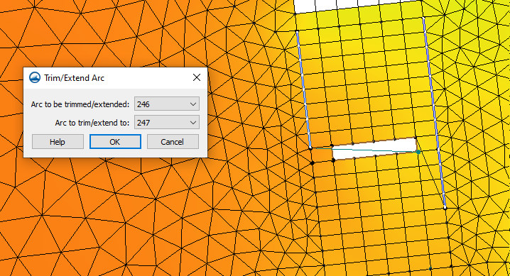
  2. Right-click and select the Extend or Trim Arc command to open the Trim/Extend Arc tool.
  3. In the tool, there are two different options: one to select the arc that will be extended or trimmed and another option to select which arc will be used as the base arc for the length.
Example of Trim/Extend Arc in SMS

There are a few ways to differentiate between wether you are extending or trimming an arc. With the extend option, the number of intersections included in the arc selection will indicate to the tool to use the "extend" operation. Whereas with the trim option, if one or more intersections are included in the selection, this indicates a "trim" operation. This will allow a node to be inserted into the first arc at the first intersection and delete the first portion of the newly split arc.

It should be noted that you can only select up to two arcs otherwise the option to trim or extend will not appear. Try trimming or extending arcs in SMS 13.2 beta today!

Blog tags: 

Using the UPW Package for MODLFOW-NWT

Do you have a groundwater model that might benefit from using the UPW package in GMS? The Upstream-Weighting (UPW) package is one of the four available options for flow packages for MODFLOW. It is used for calculating intercell conductances in a different manner than is done in the Block-Centered Flow (BCF), Layer Property Flow (LPF), or Hydrogeologic-Unit Flow (HUF) packages.Rather than the discrete approach of drying and rewetting that is used by the BCF, LPF, and HUF Packages, the UPW package treats nonlinearities of cell drying and rewetting by use of a continuous function of groundwater head.

Example of the UPW Package dialog

In order to use the UPW, you first need to have a MODFLOW-NWT simulation as part of your groundwater model in GMS. Once you have selected the MODFLOW-NWT version, you can use the Packages dialog to activate the UPW package.

The UPW flow package is based on the LPF package but differs in that the rewetting and vertical conductance correction options are not available. Otherwise, the UPW package allows you to work with both confined and convertible layers. It also has options for vertical hydraulic conductivity and interblock transmissivity. Array values can be set for the horizontal hydraulic conductivity, and vertical and horizontal anisotropy using the MODFLOW array editor in GMS.

Additional options are also included here. It is possible to remove vertical leakance correction or set a head value for dry cells. These options are in their own dialog accessible through the main UPW package dialog.

It should be noted that the UPW flow package is only available for use in the MODFLOW-NWT model and is not available with other versions of MODFLOW. The UPW is designed to work with the NWT linearization approach which generates an asymmetric matrix.

If you have a MODFLOW-NWT groundwater model that needs a different approach to calculating conductance, try out the UPW package in GMS today!

Blog tags: 

Curve Number Values for NLCD Land Use Data

Are you wondering what values to use for composite curve numbers used with NLCD land use data in your WMS project? WMS contains a Compute GIS Attributes calculator in the Hydrologic Modeling Module that allows you to import composite curve numbers to use in land use mapping. This can allow you to define boundaries for different soils, rainfall depths, etc. This post will cover some different resources to get the values you need.

Compute GIS Attributes with Imported Curve Data

It is important to be aware that there are two options when using the Computing GIS Attributes calculator: WMS Coverages as well as GIS Layers. With both GIS Layers and WMS Coverages you are given the option of selecting the Soil Layer Name, Drainage coverage computation step, etc. In the GIS Layers you are given the option to view field records and assign a code of your choosing. To use the GIS Layers option, you will need to have already imported GIS data into your project. In order to make the WMS Coverages option active you will need to have created your own land use or soil type coverages within WMS. Using the WMS Coverage option allows you to import your own land use or soil curve numbers from a text file.

What values you use for the text file depends on your own judgment and what would work best for your project. One option to get the table values is to use the example files found on XMS Wiki in the SCS Curve Numbers section. Opening one of these examples will show you an area-weighted average of the different curve numbers for the different regions. Another option is to visit the USGS website, download the example data, and import it into the GIS Attributes dialog. Finally, you can make your own table In which case use your engineering judgment to determine the CN values for your project.

Try out inserting curve number values for NLCD land use data in WMS today!

Blog tags: 

Merging Map Coverages in SMS

Do you have an SMS project that might benefit from merging coverages together? It’s not uncommon to have feature objects on different map coverages in SMS that would be useful to have on one coverage. For example, you might have feature objects from a shapefile on one coverage that you would like to merge with feature objects you have created on another coverage. This post will cover some tips to merge coverages as well as the effects of merging coverages.

To merge map coverages:

  1. Select one coverage in the Project Explorer then hold down the Ctrl key and select another coverage.
  2. Next right-click and the Merge Coverages command will appear.
  3. After clicking the Merge Coverage command, a warning dialog will ask you if you want to keep or delete the coverages being merged.
  4. Upon completion a new merged coverage will appear in the Project Explorer.
Example of Merging Map Coverages in SMS

Merging coverages comes with a lot of benefits when working with a large number of feature objects. When merging coverages here are a few items to keep in mind:

  • When merging coverages of different types, the new merged coverage will be converted to the Area Properties type.
  • When merging coverages of the same type, the new merged coverage will be the same type. For example, if you had two map coverages that are both ADCIRC materials they are going to remain ADCIRC Materials after they have been merged together.
  • When merging, only the feature objects will be merged together–any defined attributes on the feature objects will be reverted to the default setting for that coverage type. For example, the default for SRH-2D boundary conditions coverage type is the wall boundary condition. When two SRH-2D boundary condition coverages are merged all the arcs will be set to have the wall attributes.
  • When only wanting to copy a few feature objects from one coverage to another, use the Copy to Coverage feature instead of merging entire coverages.

These are just a few tips to help with merging coverages in SMS. Try out merging coverages in SMS 13.2 today!

Blog tags: 

Defining UGrids Layer Attributes in GMS

In your groundwater model, do you need to define MODFLOW-USG attributes for a UGrid that vary by layer? For example, you might have multiple polygons that define your recharge zones for your model where the attributes on each polygon are only meant to be applied to specific layers on the UGrid. GMS provides tools for specifying how those attribute definitions get applied to UGrids.

First, you can always apply attributes directly to a UGrid using the grid approach. Doing this has the advantage of having direct control over the attributes assigned to each cell and element on each layer. However, doing this on a large UGrid or for more complex models, this can become tedious and time consuming. Using the conceptual model can aid in managing assigning attributes to layers in more complex models.

For the conceptual model approach, the Coverage Setup allows you to specify the layer range for sources, sinks, boundary conditions, and areal properties. The Layer range option must be turned on in order to specify the layer range for attributes applied to feature objects in the coverage. If Layer range option is not applied then the default layer range will be used when applying attributes on the coverage to the UGrid.

Example of Specified Layer Ranges in the Attribute Table

It should be noted that once you have chosen to assign attributes to specific layers, you will need to pay attention to which attributes are being assigned. It is recommended that you review the assigned MODFLOW attributes. Keep in mind that you cannot mix specified layer ranges with the default layer range. GMS does not give priority to the default layer range over the specified layer ranges and vice versa. For example, if you assign refinement attributes to a polygon to use a specific layer range, but leave other polygons on the same coverage to use the default layer range for refinement, this will likely cause issues in the model run or results.

GMS allows you to be as general or specific as you need when assigning MODFLOW attributes to UGrid layers. Try out defining the layer attributes for UGrids in GMS today!

Blog tags: