Aquaveo & Water Resources Engineering News

Viewing Mesh Quality and ARR Plots

After generating a mesh in SMS, we hope the mesh has everything you need for a project and nothing else needs to be done for the mesh. While this is often the case, some meshes do not generate as nicely as we would like. There might be small areas where solution variables change rapidly or spots with too many connecting elements.

Quality issues in a mesh can cause issues with the model results, so you can save a lot of time by reviewing the mesh quality before running your simulation.

SMS provide a number of tools for evaluating the mesh quality. Two of these tools are the Mesh Quality Display Options and ARR Plots.

Mesh Quality Display Options

After you’ve generated your mesh, one of the fastest ways to see the quality of the mesh is to turn on the Mesh Quality Options in the Display Options menu. To do this:

  1. Open the Display Options dialog
  2. Go to the Mesh tab and turn on the Mesh Quality option
  3. Click the Options button to change how the various mesh quality checks are displayed

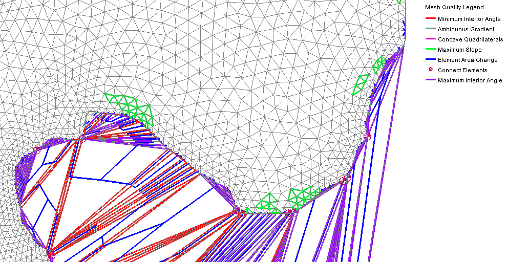
After turning on the mesh quality option, you will be able to more clearly see where there are potential quality issues. Each quality issues has its own color or symbol which is displayed in the legend. Looking over the mesh, it can become clear where there are potential issues.

ARR Plots

An Area Representation Region (ARR) plot can help you assess the overall quality of the mesh. To create an ARR plot:

  1. Select the mesh you want to review
  2. Open the Plot Wizard
  3. Select the ARR Mesh Quality option from the list on the left and click Finish

When the ARR Plot has been generated, you can use the plot to see the mesh quality.

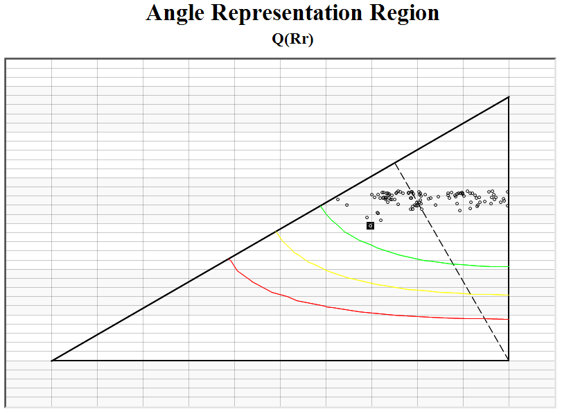
The plot has a point for each element. Points above the green line are good elements. Points below the red line are elements that should be reviewed and fixed. Points between the green and red line are elements that should be reviewed to see if they should be fixed.

Clicking on a point in the ARR plot will highlight the corresponding element on the mesh in the Graphics Window.

Try these options out in the SMS today!

Blog tags: 

Using Contours to View Contaminant Flow into a Well

You’ve finished creating a model tracking the contaminant flow into a well. Your values look good and you’re certain the model executed successfully. The only problem is that when you look at you model, the visual representation of the contaminant flow is rather lackluster. You can tell there is flow towards the well, but it’s hard to clearly see how much of the contaminant is entering. Knowing this information can sometimes make a significant difference.

The solution to this dilemma is to adjust your contour options. In particular, two options will help you see the contaminant flow more clearly: adjusting the contour interval and adjusting the contour range.

Contour Intervals

When looking at your contaminant flow, it might appear as though the contaminant has not reached your well. This can be misleading if looking at the model zoomed in and with a small contour interval. Smaller amounts of the contaminant might have reached the well, but we wouldn’t know because the interval is too small to show that level of detail.

After turning on contours for the solution set, increase the intervals around the well by doing the following.

  1. Zoom in on the well area.
  2. Make the contaminant dataset active in the Project Explorer.
  3. Click the Contour Options macro.
  4. In the Dataset Contour Options dialog, increase the contour interval value.

Now the contour has been broken up into more intervals, making it easier to see when the contaminant first reaches the well.

Contour Ranges

Another option is to change the contour range so it targets the values near the well. After turning on contours for the solution set, change the range by doing the following.

  1. Zoom in on the well area.
  2. Make the contaminant dataset active in the Project Explorer.
  3. Click the Contour Options macro.
  4. Turn on the Specify a range option.
  5. Enter minimum and maximum range values that focus on those contour values near the well.

Now the contours specifically highlight the contaminant flow into the well.

By experimenting with the different contour options, you can find the one that best shows contaminant flow in your project. Try this today in GMS!

Blog tags: 

3 Ways to Troubleshoot WMS Basin Issues

Have you noticed your model’s basin isn't what you hoped it to be? When you create a solid watershed model, there are a few common issues that can make the model not work as intended. These include:

  1. Having a flow accumulation threshold that is too low or too high.
  2. Having one or more outlets in the wrong location for proper definition of the sub-basins and basins.
  3. Trying to work with a project area that is too large or too small for the intended purpose.

Flow Accumulation Threshold

Setting the correct flow accumulation threshold is very important. If you set the flow accumulation threshold too low, it may not accurately show the information you need, leaving sections of the watershed model reporting dry conditions. If you set it too high, you can be overwhelmed with too much information. It is good practice to try multiple levels to see which provides the most accurate results for the project. You can adjust this setting by doing the following:

  1. Open the Hydrological Modeling Wizard dialog.
  2. Select Compute Flow Directions and Accumulations (TOPAZ) from the list on the left.
  3. Enter the desired Min flow accumulation threshold and close the dialog.

Adjusting the Outlet

Placing an outlet in the wrong location causes the entire structure of the stream system to change dramatically. This can produce sub-basins quite different than desired, which can lead to results not lining up as expected. Remember that everything upstream from an outlet will be part of the same sub-basin or basin, so be careful when placing your outlets for each sub-basin as well as for the full basin.

Project Area

Sometimes, you may select a larger area than necessary for your model, or you may select an area too small for the project to produce useful results. If the area is too large, the desired details may not show up in your results. If the selected area is too small, you may not have enough data on which to base your decisions for the watershed.

If you keep these ideas in mind, your watersheds will better represent the areas you're modeling. Experiment with this today in the WMS Community Edition.

Blog tags: 

Stockholm GMS Training 2018

Aquaveo recently taught a three-day GMS training session hosted by the School of Engineering Science at the KTH Royal Institute of Technology in Stockholm, Sweden. The institute’s Prosun Bhattacharya arranged and coordinated the training session.

From May 15-18, 2018, Alan Lemon and Hoang Tran presented on a wide range of topics, including general groundwater modeling concepts, using MODFLOW in GMS using both grids and conceptual models, incorporating field data (such as scatter point and borehole data) into a GMS project, and calibrating models in GMS. Models demonstrated and discussed include MODFLOW, MODFLOW-USG, MODPATH, MT3DMS, and SEAWAT.

Participants came from several different countries, companies, and governmental and non-governmental organizations, including:

There were also graduate students from Gdańsk University of Technology in Poland, and KTH Royal Institute of Technology and Luleå University of Technology in Sweden.

After the classes, Alan and Tran enjoyed walking around Stockholm and seeing the sights, including the Vasa Museum and the Nobel Museum.

Aquaveo provides custom, on-site training for SMS, GMS, WMS, ArcHydro Groundwater, and any other water resource modeling need you have. Organizations can set up shared trainings such as this one, or arrange for the same training for their own employees. You can learn more about our training offerings by visiting our site.

Blog tags: