Aquaveo & Water Resources Engineering News

Avoiding Grid Over Refinement in GMS

When building a grid for your groundwater model, it can certainly be tempting to make a really refined grid. While this temptation is understandable, there are certain pitfalls that can result from having a grid that is overly refined. This post will go over some of the reasons to avoid overrefining your grid in GMS.

There are, of course, legitimate reasons to refine portions of your grid. Portions of the grid that are key areas should be refined. This should be done only in areas around wells or other structures that are important to the model. By refining key areas, important areas of the grid will receive more attention during the model run. However, over refining your grid can cause some issues, including some of the following ones listed here.

Example of Grid Refinement

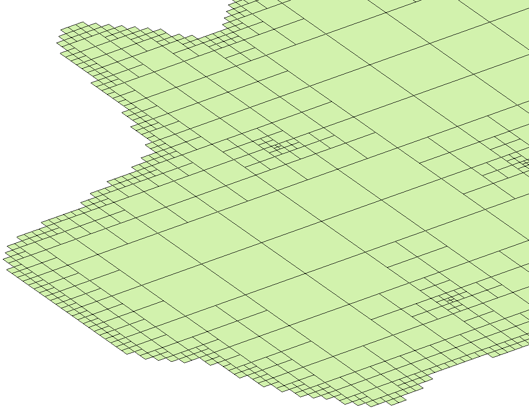
When you are refining, you are creating more grid cells in your grid. Each of these cells will be used in the model run calculation. A grid that has been over refined generally has a lot of cells that need to be used in the model calculations, many of which are unnecessary. This will cause the model run to go slower and take longer than the same model without the over refinement.

Because an over refined grid contains refined cells in unimportant areas of the project, the data from these areas can sometimes skew the results. The model run does not generally discriminate between important and unimportant parts of the grid. When it encounters a portion of the grid that has a lot of cells, it gathers all the data it can for that area. In an over refined grid, this can mean it gathers more data than the model needs, which sometimes can skew the results.

The biggest issue we most often see is when over refined grids cause the model to fail to converge. Once again, an over refined grid will have too many cells and be collecting too much nonessential data. All of this can overwhelm the model and can cause the model run to diverge. To resolve this, you will need to simplify the grid so that the model run stays focused on the key areas of the model.

Try out some of these tips while refining grids in GMS 10.5 today!

Blog tags: 

World Bank ArcHydro Groundwater Training

Recently, Aquaveo had the opportunity to participate in an ArcHydro Groundwater training organized by the World Bank. The online training happened from the 9th to the 12th of November 2021.

AHGW example

The training covered the uses and applications of the ArcHydro Groundwater (AHGW) tool used with ArcGIS. AHGW aids in displaying and analyzing multidimensional groundwater data, including representations of aquifers and wells/boreholes, 3D hydrogeologic models, temporal information, and data from simulation models.

Topics covered in the 4-day training included setting up a groundwater model and working with boreholes data. Other topics covered further included creating wells and cross sections in groundwater models, along with performing model analysis.

The training had 30 active participants in attendance from the National Water Informatics Centre (NWIC), the National Hydrology Project (NHP), the National Institute of Hydrology (NIH), the Water Resources Department (WRD) of the Indian Institute of Remote Sensing, and ESRI. For the online training, participants were located in various states in India including: Kerala, Karnataka, Uttar Pradesh, Tamil Nadu, Sikkim, West Bengal, Odisha, Telangana, Maharashtra, Gujarat, and Rajasthan.

Aquaveo would like to thank the World Bank for setting up this online training. We'd also like to thank all of the participants for their interest and efforts in using AHGW.

If you are interested in attending a training session for AHGW or any of Aquaveo's products, check out our training page for upcoming training sessions. Training sessions can be either in-person or online. Additionally, you can request a training session from Aquaveo by contacting our consulting team.

Blog tags: 

Plotting Observed Data onto a Computed Time Series Plot

Have you been wanting to make a direct graphical comparison of observed time series water-level data with computed time series water-level data? Have you been hoping to use data observed in the field to help calibrate your 2D hydraulic model in this way? While not officially supported yet, we have a workaround that could potentially help with this. This post will review how to plot both observed and computed water-level data onto the same time series plot.

There is no direct method for plotting observed data onto a computed time series graph. However, the following workflow should be able to suffice as a solution:

  1. From within SMS, bring up the File Import Wizard by using File | Open to select the file for your observed time series data.
  2. On Step 2 of the File Import Wizard, set the SMS data type drop-down to "Scatter Set", and once properly configured, click Finish to close the File Import Wizard and import the observed time series data into SMS as a scatter set.
  3. Once the data has been imported, interpolate the scatter set to your mesh by right-clicking on the scatter set and selecting the Interpolate to... command to bring up the Interpolation Options dialog.
  4. Select the scatter set data you would like and the mesh you would like to interpolate the data to, and click OK to close the dialog and interpolate.
  5. Click the Plot Wizard macro to bring up Step 1 of the Plot Wizard dialog.
  6. Select "Time Series" from the Plot Type list and click Next > to move on to Step 2 of the Plot Wizard.
  7. Select "Use selected datasets" and then click the All Off button underneath it. This will now allow you to select which specific datasets you would like to appear on the graph.
  8. Click Finish to close the Plot Wizard and bring up the Plot Window. The graph you have specified should appear.
  9. To further modify the graph, right-click on it and select Plot Data... to bring up the Data Options dialog. This will allow you to get back to the previous options and change your selection of datasets.
Example of a plot combining observed data in a computed time series plot

A future version of SMS may incorporate a more direct method for this process. But don’t let that stop you from trying out plotting observed data onto a computed time series plot in SMS 13.1 today!

Blog tags: 

Using the Axes Display in GMS

Have you tried using plotted axes to help orient the display of your models in the Graphics Window for your groundwater modeling projects in GMS? Within the Display Options in GMS, there is a set of options that will allow users to activate this and modify how it will display. This post will review how to utilize the Plot Axes functionality found in the Display Options dialog within GMS.

To locate the Axes options in GMS, open up the Display Options dialog by doing the following:

  1. Click the Display Options macro or go to the Display | Display Options... command.
  2. Select the Axes option on the left.
  3. Turn on the checkbox labeled "Enable axes" to activate the plot axes.

By default, the axes are turned off, and all the other options below it grayed out as a result. This is why axes are not usually visible on their own in the Graphics Window. Turning this option on will generate axes within the Graphics Window. The axes will naturally be sized to contain the entirety of the model within it. If the Graphics Window is currently set to Plan, Front, or Side View, rotation might be required for all of the axes to be visible.

Example of the Axes Display Options

The Axes display options allow you to control the different aspects of the axes display, such as:

  • Fly modes to set where in space the axes will be placed.
  • Tick location options to set which direction tick lines along the axes will be drawn pointing to, either inward or outward.
  • Grid line location options to set which surfaces grid lines are actually drawn on, which can help in visualizing the grid.
  • A spreadsheet containing options for editing each individual axis, as well as a row for editing all of them at once.

Try out experimenting with Axes display options in GMS 10.5 today!

Blog tags: