Aquaveo & Water Resources Engineering News

Incorporating Geology into a MODFLOW Model

Have you created a MODFLOW model and would like to incorporate geological features in between the MODFLOW layers?

The first step is to create the solid to be used. In GMS, solids are representations of stratigraphy used for site characterization and visualization. Solids can be created in any one of three ways:

  1. Convert horizons to a solid.
  2. Convert one or more TINs to a solid.
  3. Manually create a solid by right-clicking in the Project Explorer and selecting the desired type of solid from the New | Solid menu.

Using the first two methods will allow the solid material composition (what the solid is made of) to be automatically interpolated from the horizon or TIN information. Using the third method will allow you to select the material for each solid reated. The third method also requires knowledge of the XYZ coordinates and other attributes, depending on the type of solid being created (cube, cylinder, sphere, or prism).

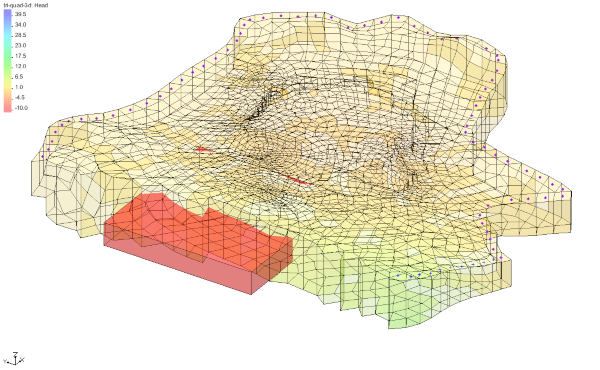
Once you’ve created your solids, these steps will integrate the solids into the MODFLOW model:

  1. Right-click on the grid and select Classify Material Zones… to bring up the Classify Material Zones dialog.
  2. Select the solids folder you just created.
  3. Select the Classify algorithm you want to use.
  4. Enter the name of the material set being created.

The Centroid algorithm assigns the solid to the cell if it passes over the centroid of the cell. The predominant material algorithm assigns the solid to the cell if it is the predominant material in the cell (the material making up the highest percentage of the cell). This method maintains your grid, while interpolating the materials to the grid, so that you can have multiple materials within a layer.

Try adding solids to your MODFLOW models in GMS today!

Blog tags: 

Working with Rain Gages in GSSHA

Are you needing to add rain gages to your GSSHA model? Using rain gages to define your precipitation in GSSHA is extremely useful due to its ability to spatially model precipitation over a watershed. Combining spatially varying rainfall with the distributed parameters of GSSHA is a great way to create a fairly realistic model for your watershed.

One of the bigger challenges when simulating a storm event is finding reliable data. Although it is important to investigate the most accurate source for your particular watershed, there are websites containing NOAA and GLDAS data for not only the United States, but globally. Having many sources of compiled data all on one site makes Cuahsi’s HydroClient a very useful resource. For those using our software internationally, another possibly useful resource when gathering storm data from the Global Precipitation Climatology Centre. This gives monthly values from 1901-2013, with newer data being added frequently.

Now that you have solid data for your watershed, it is time to define your gages. To use rain gages as your precipitation input:

  1. Create a rain gage coverage.
  2. Create rain gages in their proper locations.
  3. Using the Select tool, double-click on the gage to bring up the Rain Gage Properties dialog.
    1. Set the gage type to GSSHA.
    2. Define the precipitation using either a cumulative or an incremental distribution.
    3. Beneath the Show drop-down, choose GAGES if your data is incremental, and ACCUM if your data is accumulative.
  4. Return to the 2D-Grid module and select GSSHA | Precipitation.
    1. Select Gage as the rainfall event, select Rain Gage, and choose your preferred interpolation method (Inverse distance weighted or Thiessen polygons).

For more information and specifics on working with gages in GSSHA, please take a look at the GSSHA user’s manual. WMS provides a useful and helpful resource when creating a GSSHA model, analyzing and viewing the results. Practice using rain gages as your precipitation source in WMS 11.0 today!

Blog tags: 

New Bridge Scour Tool in SMS 13.0

You are probably aware of the potential destruction caused by bridge scour. Up to 60 percent of bridge failures in the United States from 1950 to 1989 were caused by scour. Bridge scour occurs when the stream bed material around bridge piers is eroded. This can leave the pier unsupported by the stream bed, causing it to collapse.

Recent news has shown bridges of all sizes all around the world collapsing or in danger of collapsing due to scour. Such failures can have a huge negative impact on the economy and also pose a danger to the lives of those who use the bridge regularly. The Federal Highway Administration (FWHA) advised that it is far less expensive to take measures to prevent scour than to replace a bridge that fails due to scour.

Part of the scour mitigation process is evaluating countermeasures that can be taken to prevent such failures. These include onsite surveys and inspections, physical modeling such as that done at the FWHA Hydraulics Laboratory at the Turner-Fairbank Highway Research Center in McLean, Virginia, and computer modeling using tools such as the Surface-water Modeling System (SMS) from Aquaveo.

SMS 13.0 adds powerful new post-processing Bridge Scour tools that can be used to quickly test the scour effect of different pier arrangements, pile sizes and shapes, and vessel impact protection structures such as dolphins and fender rings. The Bridge Scour feature in SMS 13.0 can be used with the FWHA Hydraulic Toolbox to take advantage of its various bridge scour calculators and mapping tools.

One of the most exciting features of Bridge Scour is how it saves time. When creating the contracted section, approach, centerline, bank, abutment toe, and pier arcs, SMS 13.0 automatically assigns the arc type if they are created in order. This translates into saved time and cost, allowing you to be more productive.

Check out the Bridge Scour tool in the SMS 13.0 beta.

Blog tags: 

Troubleshooting MODFLOW

Are you experiencing issues with your MODFLOW simulation? Unable to get your model to converge? Even after properly constructing a model in GMS, you might still find that your model won’t converge or it terminated with an error. Below are some hopefully helpful suggestions on why the model might not be converging and what you can do about it.

To begin, look at what might be causing the convergence issues to occur. The model might have improper aquifer properties which should be reviewed and adjusted if needed.

Another possibility is that there is an unbalanced flow budget. An unbalanced flow budget can manifest itself in two ways. One way is when the inflow is greater than the outflow, then the model can experience sometimes extreme flooding, and the model in turn will not converge. The other way in which there can be an unbalanced flow budget is if the outflow is greater than the inflow. If all the cells in a model are caused to go dry, then the model will not converge. A high outflow may be caused by things such as high conductivity and high pumping rates.

Another possible issue that might cause MODFLOW to have some issues is if you have a specified head for all grid cells in the model. This is because when all cells are Specified Head boundaries, then there is nothing for MODFLOW to compute and the model will terminate with an error.

Some other common issues include: improper initial conditions, improper boundary conditions, wetting and drying issues (as mentioned above) and a highly sensitive model. If the area is known to be highly sensitive, this might cause MODFLOW to not converge due to the speed at which flow can be affected.

Now that we know of some issues which might cause MODFLOW to struggle, we can take a look at three basic troubleshooting steps.

Basic Troubleshooting Steps:

  1. Review the command line output from MODFLOW, and check to see where the issue began to arise. This will enable you to better pinpoint the cause of the error.
  2. Before running MODFLOW, make sure you always run the model checker to see if there are any errors that will prevent convergence. Immediately repair the errors found in the Model Checker. The Model Checker can be found by clicking MODFLOW | Check Simulation…
  3. Look in the MODFLOW output file (*.out) to search for missing values.

Further detail for some specific issues is also given below.

  • If the head is going to drop below the cell, use the MODFLOW-NWT solver.
  • Cells usually go dry due to a low recharge or a high conductivity. Adjust these parameters to better calibrate the model.
  • A transient water table will cause a fluctuation in the heads and the cells may go dry. In this case it is best to use the rewetting option which is available in all flow packages. However when possible MODFLOW-NWT is still the best solution to this problem.
  • Relax the maximum residual or head change criteria. It is best to not increase these values beyond about 1% of the value.

Hopefully with these troubleshooting tips, you can get your MODFLOW simulation up and running in no time. Additional information can be found in the Frequently Asked Questions section of the MODFLOW user manual under the question "My model hasn’t converged. What can I do?" If you are still struggling to get your model to work, consider using Aquaveo's consulting services for expert assistance.

Blog tags: 

How to Calculate Riprap Using the Hydraulic Toolbox

Are you needing to determine the size of stones needed for riprap? Having stones that are too small will reduce the effectiveness of the riprap which could be disastrous. On the other side, having stones that are too large could cause unnecessary expense.

After defining drainage data in WMS, it is possible to calculate the riprap needed for your model using the FHWA Hydraulic Toolbox. To do this:

  1. Define your drainage data in WMS.
  2. Assign each basin attribute to an analysis method by double-clicking on the feature, and then selecting Edit Attributes…. This will give you the opportunity to link your drainage data to the Hydraulic Toolbox.
  3. Click on the Hydraulic Toolbox macro in WMS to bring up the Hydraulic Toolbox.
  4. You can calculate riprap using one of two methods:
    • Channel Lining Design Analysis Tool. Keep in mind when using this tool that a filter material must be separately designed.
    • Riprap Analysis Tool. This tool will calculate the filter material along with riprap size.

Once in the Hydraulic Toolbox, locate the name of the analysis method chosen and double-click to open the analysis dialog for the chosen parameter and method. You will notice that all of the data you input into WMS is now filled in the analysis tool. After you specify blank parameters, the tool will calculate and display the results at the bottom of the screen under “Minimum Riprap Thickness”.

Using the Hydraulic Toolbox to calculate riprap can help your project move forward. The toolbox also contains many other features worth exploring. Try using the Hydraulic Toolbox today!

Blog tags: 

Aquaveo Visits Namibia

From November 6-9, Aquaveo had the privilege of traveling to Windhoek, Namibia to conduct a training and provide consulting sponsored by BGR for several employees of MWAF. The Ministry graciously provided space in its building for the training classes. During the training classes, Alan Lemon helped them refine a MODFLOW model of the Ohangwena II aquifer.

Northern Namibia has a long history of droughts, and Namibia is the driest country in sub-Saharan Africa. Surface water is not a reliable source for potable water in the area due to the infrequency of rain storms to replenish the watershed. Because of this, the Namibian government—through its Ministry of Agriculture, Water, and Forestry (MWAF)—partnered in 2012 with the German Federal Institute for Geosciences and Natural Resources (Bundesanstalt für Geowissenschaften und Rohstoffe, or BGR) to research and develop an aquifer discovered near the northern border with Angola.

The Ohangwena II aquifer is found below an area about 75 km by 40 km, and has nearly 20 billion cubic meters of fresh water. This is enough to last for well over 400 years at current usage levels, and some think there may be even more water there. This kind of resource would be invaluable to the Namibian people.

Creating a valid working model of the aquifer will help the government of Namibia and BGR to come up with a solid groundwater management plan. Such a plan will help them better manage this amazing resource so that the people living in northern Namibia will have the water they need while also preventing needless wasting of hundreds of years of water located in the precious aquifer.

During the trip, Alan had the chance to visit the Okaukuejo Waterhole in Etosha National Park, where he saw a number of different animals, including rhinoceroses, crocodiles, and springbok. The watering hole is visited by tens of thousands of animals each year, from small birds and mammals to some of the largest and most dangerous animals in Africa. The national park is near the area covered by the Ohangwena II aquifer.

We want to thank BGR and MAWF for inviting us to their facility, and for the opportunity to work on such an important project. If you are interested in having Aquaveo assist with your projects, check out our consulting services.

Blog tags: 

New Floodway Delineation Tool in SMS 13.0

City planners, developers, and others have a great interest in using available land. Sometimes that land is close to areas that flood, so precautions need to be taken so the build site is not too close to (or directly in) the potential flood area. Failure to properly plan and delineate a floodway can potentially cause millions of dollars in flood damage as well as potential losses in property values. Hurricanes Harvey and Florence, with their extreme rainfall amounts, are prime example of why floodway delineation is so important.

In addition to the guidance provided by the Federal Emergency Management Agency (FEMA), the new Floodway tool in SMS allows the extents of a floodway area to be more clearly defined. This tool allows planners, developers, and others to run multiple simulations to determine the safest places to build as well as the places which may be most impacted during a significant flooding incident.

To use the Floodway tool in SMS, a project must have a either a Cartesian grid, a 2D mesh, or a 2D scatter set that has simulation result datasets for at least water depth and velocity. Two coverages are also required: a 1D hydraulic centerline coverage and a 1D hydraulic cross section coverage.

The way the Floodway tool works is by calculating how far in from both sides of a river or stream that vertical walls can be placed and raise the center of flow by the targeted maximum rise. FEMA suggests this rise should be no more than 1 foot. These calculations use the input provided by the water depth dataset, the velocity dataset, and the two hydraulic coverages to define the floodway extents along the entire length of the study area.

Once these extents are known, the data can be used when making area planning and development decisions at all levels of government and businesses. You can try out this feature in SMS 13.0 beta today.

Blog tags: 

New and Improved Lidar Tools in GMS 10.4

With the release of GMS 10.4 (beta), a set of new and improved tools for importing and handling lidar files is now available. The new tools provide much faster import times, and most processing happens on the fly as the lidar display options are adjusted.

Merging and Display Options

As with previous versions of GMS, either a single or multiple lidar files can be imported. However, the options available for handling the lidar data have changed significantly, offering more precise control and more options that will allow better use of the lidar file data.

One of the best new features is that GMS 10.4 allows merging multiple lidar files into a single file. This is accomplished by selecting the desired lidar files in the Project Explorer, then right-clicking and selecting Merge. Enter the desired filename and allow GMS to process the merge.

After the merging is complete, you can import the new lidar file into your project.The merged file has all of the lidar cloud points that were contained in the original lidar files, though not all of them may be visible. The visibility of lidar cloud points can be adjusted using the display options for the merged lidar file. Access them by right-clicking on the merged lidar file in the Project Explorer and selecting Display Options… to bring up the Display Options dialog.

]

This dialog allows you to change point size, how many are displayed, which kinds are displayed, which points to exclude, and how to exclude them. This allows you to choose the level of complexity without overwhelming you with too many options. The following image shows the merged lidar file with 5 million points displayed.

Interpolation Options

  • UGrid: If your project has an existing unstructured grid (or one that has been imported or created), you can interpolate the lidar files to that UGrid. Simply select the desired lidar files in the Project Explorer, then right-click on them and select Interpolate to UGrid… to bring up the Interpolate Lidar to UGrid dialog. This allows you to select the target UGrid, set the new dataset name, and set the sampling distance.
  • Raster: This option uses the lidar display options set at the time of interpolation and creates a raster file. The Interpolate Lidar to Raster dialog allows the number of X and Y cells to be set, and changing those affects the cell size. The merged raster is then imported into the Project Explorer.

Try these new features today in GMS 10.4 (beta).

Blog tags: 

Quickly Delineating a Floodplain

How many watershed projects require knowing which areas are in a floodplain? There is a lot of debate over building on floodplains, but before that debate can happen, the location of the floodplain needs to be known.

A new feature in WMS makes this process quick and simple.

The Map Flood tool utilizes ground elevations and existing flood hazard maps from the Federal Emergency Management Agency (FEMA) to quickly visualize the impacts of possible modifications in the flood level. The tool is designed to utilize data from web services including ground elevations, flood hazard base flood elevations, and flood hazard floodplain extents.

The Map Flood tool is accessed by clicking on the Map Flood icon in the toolbar.

Running the tool will do the following:

  • Download elevation data for the area which is stored as a scatter set
  • Download base flood elevation lines for the area which is stored as a map coverage
  • Download a flood extents polygon which is stored as a map coverage
  • Download a flood insurance map as a image in the GIS module
  • Create a water surface elevation for the base flood
  • Create an offset water surface elevation for the modified flood level
  • Compute a new flood extent polygon for modified flood level

For locations that do not have FEMA data, you can use your own data to generate flood extents. As long as a ground elevation dataset and a water surface elevation have been imported into a WMS project, then the Map Flood tool can be used to create a fast floodplain. This data needs to be imported into WMS as either a 2D scatter set or a TIN.

Using the new Map Flood tool can greatly reduce the time it takes to delineate a floodplain. Try out the new Map Flood tool in WMS 11.0 today!

Blog tags: 

What We Learned at the 2018 Aquaveo User Conference

Aquaveo held its first annual User Conference from October 16-17, 2018! It was amazing to get to meet so many of our users at once. We hope everyone had a great time.

For us, it was exciting to meet users from all over the world. We met users from the United States, Canada, Portugal, Germany, the United Arab Emirates, Guyana, and Thailand. When asked why they came, the attendees said they came to learn:

  • How Aquaveo’s products can help with their projects
  • More of what Aquaveo has to offer
  • What Aquaveo is all about

In listening to what our users had to share with us, we took away a couple key items that you want to see improved in our software.

  1. You want modeling to go faster. We understand the demand to give results in less time is growing, so we will be looking at ways to make the process of modeling take less time and still be accurate. Some of the innovations added into Aquaveo’s software already significantly reduce the time it takes to complete a model. We hope to add more automation and tools to speed up modeling times.
  2. You need to be able to work with big data. More data is becoming available and you want to be able to use it. This means processing large files covering larger areas in more detail. At Aquaveo, we are working on doing this, including optimizing our code and adding new tools to work with large files such as lidar files.

We’d like to thank the following for participating in our user conference:

If you couldn’t make it to the Aquaveo User Conference this year, we will be having another one next year. Watch our website and Facebook page for future details. See you next year!

Pages