Aquaveo & Water Resources Engineering News

Using the MODFLOW HFB Package

Sometimes in a MODFLOW simulation, you need to simulate very thin barriers to flow that aren't accurately represented by assigning values to entire cells. Fortunately, MODFLOW has the Horizontal Flow Barrier (HFB) package that facilitates accurately modeling thin flow barriers. Today, we explore how the HFB package can meet your needs, and how it functions.

The HFB package can meet your need for a more realistic approach to simulating horizontal barriers in your model. Whereas many packages in MODFLOW assign values to entire cells, that might poorly reflect reality for horizontal flow barriers with negligible width. These barriers might include slurry walls, sheet pile walls, or diaphragm walls around wells. Instead of assigning values to whole cells, the HFB package uses cell boundaries to simulate horizontal barriers. Doing so can more accurately reflect the actual situation.

To use cell boundaries to simulate horizontal flow barriers, the HFB package uses a hydraulic characteristic. You calculate the hydraulic characteristic by dividing the hydraulic conductivity of the barrier by the real-life width of the barrier. This value is assigned to cell boundaries. Then, MODFLOW uses that value to modify the regular flow between cells. Thus, you get modified flow at the cell boundaries that have a defined hydraulic characteristic.

Example of the HFB Package in GMS

The following is a suggested workflow for using the HFB package:

  1. Make sure that the HFB package is turned on in the MODFLOW Packages / Processes dialog.
  2. Set up a coverage that can include a barrier by checking Barrier in the Coverage Setup. Define the layers that the barrier affects using the Default layer range in the Coverage Setup.
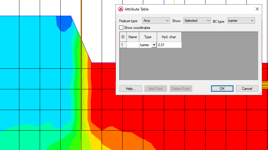
  3. Draw an arc representing the barrier. In the Attributes table for that arc, set its boundary condition to "barrier". Define its Hydraulic characteristic as you have calculated it.
  4. Map from that coverage to MODFLOW.

The values for the HFB package can be edited using the HFB - Horizontal Flow Barrier command in the MODFLOW menu.

While using the HFB package, keep the following in mind:

  • There are certain assumptions that this package uses to function. It's assumed the barrier has no storage capacity. It's also assumed the barrier has negligible width. Therefore, the HFB package's sole function is to reduce conductance between adjacent horizontal cells.
  • This blog post primarily applies to standard MODFLOW versions. The HFB package is also available for MODFLOW 6.

Try out the HFB package in GMS today!

Blog tags: 

Computing a Courant Number for an SRH-2D Model

Sometimes, you might want to calculate a Courant number for your SRH-2D model. In most cases, this isn't necessary because SRH-2D is an implicit model. Unlike explicit models such as HEC-RAS, SRH-2D is not Courant limited. With SRH-2D, it is more important to verify convergence and stability than Courant compliance. However, we know that calculating a Courant number dataset for SRH-2D is occasionally desired. Fortunately, SMS now has the Advective Courant Number tool to compute a Courant number dataset based on velocity.

First, let's be clear about what a Courant number does. A Courant number tells you the number of mesh elements that a given water particle passes through during a time step. If the Courant number is less than one, the given particle of water would not pass through an entire mesh element in a single time step.

In SMS, the Advective Courant Number tool computes a Courant Number dataset including every node at every time step. It uses the following equation:

Courant Number Equation

To use the Advective Courant Number tool, do the following:

  1. Make sure a transient SRH-2D solution file is already loaded.
  2. Open the SMS Toolbox, and under Datasets, find the Advective Courant Number tool.
  3. Set the Velocity dataset, the time step length for the simulation, and the desired name for the output dataset.
  4. Run the tool.
Example of the Advective Courant Number tool

The Advective Courant Number tool might stall depending on the vector dataset for your SRH-2D simulation. Running the SRH-2D simulation again might solve this problem. Before running the simulation again, we recommend saving the project as a new file to preserve the old solution files. Then, in the new SMS project file, run SRH-2D again. Once the new solution is loaded into SMS, run the Advective Courant Number tool again using the new velocity dataset.

To see the results, open the Properties dialog for the Courant number dataset. There, you will find the maximum and minimum for the whole dataset and the current time step.

Calculate the Courant number dataset for your SRH-2D simulation in SMS today!

Blog tags: 

AHGW Pro for ArcGIS Pro Now in Beta!

We are excited to announce the release of Arc Hydro Groundwater Pro (AHGW Pro) for ArcGIS Pro in beta! Arc Hydro Groundwater has long helped ArcGIS users archive, display, and analyze multidimensional groundwater data. Now these same capabilities are available in ArcGIS Pro.

Arc Hydro Groundwater is a product that Aquaveo created in collaboration with ESRI. It is an add-on to ArcGIS software that enables you to work with groundwater data in ArcGIS applications. Its many capabilities include modeling boreholes and wells, creating and editing cross sections, and building 3D models.

With this new release of AHGW Pro, we wanted to highlight some of the features available.

Example of AHGW Pro

For starters, you now get to combine the geodatabase technology of Arc Hydro Groundwater with the modern interface of ArcGIS Pro. AHGW Pro contains all of the tools available in AHGW with the exception of the MODFLOW analysis tools.

Another change is that ArcGIS Pro often uses panes rather than wizards and dialogs. Panes, unlike dialogs, do not have to be closed for other work to get done in ArcGIS Pro. The AHGW tools have been converted to use this pane format. This means that a tool from an AHGW Pro toolset can run while you work on something else. Furthermore, it gives you the capacity to leave the Geoprocessing pane open. Leaving a pane open preserves the last settings used in that pane. This means you can use the Geoprocessing pane to run a tool with the same settings—or slightly modified settings—more than once without having to set all the same parameters again.

Of course, you might be wary of having a lot of panes open. Fortunately, ArcGIS Pro makes it possible to stack panes, so they are neat, organized, and out of the way. You can therefore have multiple AHGW tools open while working on your project.

See what AHGW Pro and ArcGIS Pro can do together by downloading AHGW Pro for ArcGIS Pro today.

Blog tags: 

Exporting Contour Shapefiles from a 3D UGrid

Have you ever wanted to export the linear contours on a 3D UGrid as a shapefile? By exporting GMS contours as shapefiles, you can open contour shapes in other GIS applications or in other GMS projects. GMS provides functionality for exporting UGrid contours to shapefiles. This article gives some guidance for using this functionality.

In GMS, linear contours display on the top and the bottom of the 3D UGrid. This can result in contour shapefiles with undesired shapes that make contours unclear. Fortunately, GMS 10.7 can now display just one cell face (top or bottom) of single layers in a 3D UGrid. This enables exporting cleaner contour shapefiles from one face of a layer in a UGrid.

For example, GMS can display just the top of layer 1, or it can display just the bottom of layer 3. This can make for cleaner contour shapefiles because the files will have contours from only one face of the 3D UGrid. This is useful if you want the contours from a UGrid but only need the top- or bottommost contours.

Example of exporting UGrid contours to a shapefile

Do the following to export contour lines from one face of a UGrid layer as shapefiles:

  1. Have a 3D UGrid visible in the Graphics Window. Make sure that it has a dataset that can be visualized using contours.
  2. Activate the desired dataset.
  3. Set the contours to linear in the dataset Display Options.
  4. Turn on Single layer in the UGrid Single Layer toolbar and select the desired layer. By default, the UGrid Single Layer toolbar is to the right of the XYZS Bar at the top of the GMS window.
  5. Adjust the drop-down in the UGrid Single Layer toolbar to show the cell faces desired: top, bottom, or all. GMS displays the top faces by default. This also adjusts which contours display. Now you have a certain set of contours singled out. These will be made into contour shapefiles.
  6. Right-click on the active UGrid and select Export.
  7. In the Export UGrid dialog that appears, select "Arc Shapefile of Linear Contours (*.shp)" from the Save as type drop-down and save the contour shapefile with the desired name.

If you move the shapefiles, make sure to move them with all of their accompanying files. That includes the files ending in "*.dbf", "*.prj", and "*.shx".

There may be breaks in the displayed faces of the UGrid when only showing the top or bottom face of a layer. This is because some adjacent cells are joined only by vertical cell faces; the edges of the top or bottom of the cells don't touch. Thus, when the vertical cell faces are hidden, there is only empty space. This often affects the display of the contours and the contour shapefiles.

Try exporting your UGrid contours as shapefiles in GMS 10.7 today!

Blog tags: 

Switching Model Executables

The Groundwater Modeling System, Surface-water Modeling System, and Watershed Modeling System (collectively known as XMS) applications make use of multiple numerical models. XMS is packaged with the executables for each of these numerical models. At times, you may need to switch out which numerical model executable XMS uses.

In general, you will want to use the model executable that comes packaged with the XMS. XMS is coded to work with the specific model executables that are distributed with each version of the software.

There are some reasons you might want to change which model executable it used. It might fix a bug with the model executable. It might get you access to features in an older or newer version of the model executable. It might also help you test issues with the numerical model. Replacing the model executable isn't guaranteed to help with any of these, but it is one option for troubleshooting with all of them.

For all XMS applications, the numerical model executables to be used are selected in the Preferences dialog. If you already know where the model executable is, you can copy and paste the executable into the preferences dialog. To do so, use the following workflow:

  1. Copy the executable file path. If using Windows 11, right-click on the desired model executable and select "Copy as Path."
  2. If using Windows 10, open the Properties dialog from the right-click menu. Copy and paste the location path into a text document. Then, make sure to grab the file name ending in ".exe" as well. The executable path will be incomplete without that file name.
  3. In your XMS software, open the Preferences dialog from the Edit menu.
  4. Find the model executable that you want to change and click on the file path next to the name or the Browse button.
  5. In SMS or WMS, this will bring up an Open dialog. In the File name box, paste in the new executable path. If you are using Windows 11, make sure to delete the quotation marks at the beginning and end. Selecting Open saves the new model executable.
  6. In GMS, the model executable is editable without bringing up the Open dialog. Simply erase the former executable path and paste in the new one. As long as the path is a valid path and the path ends in ".exe", GMS will save it. Again, for Windows 11, delete the quotation marks.
  7. Finalize the model executable by clicking OK to exit the Preferences dialog. Otherwise, the executable will not save.
Example of model executables in the Preferences dialog

Now, there are some issues to keep in mind. As mentioned earlier, changing out a numerical model executable is not guaranteed to fix a particular issue or even improve the situation. Older or newer versions of the model executable may not always be compatible with your version of XMS. Sometimes the model executable is not compatible with a particular project. The new executable might even worsen the situation. If any of these things happen, you can reintroduce the original executable.

Check out the available model executables in XMS today!

Blog tags: 

Exploring Display Themes in SMS

SMS has an expansive suite of display options that allows you to visualize your results with style and clarity. What’s more, SMS has tools that can streamline how you adjust display options. Have you ever wanted to be able to adjust display options in SMS without actually opening the Display Options dialog? Have you contoured a dataset to your liking and now want to save those particular contour settings to return to them quickly? Display themes make these things possible. Today we discuss the uses of display themes as well as considerations to keep in mind while using them.

Display themes have several uses. Imagine a project where you want to quickly navigate between two different parts of the project. Display themes can be used to save view options, so you can jump back and forth between opposite ends of the project by clicking on the display theme in the Project Explorer.

Example of Display Themes in SMS

Display themes also allow you to develop a unique set of contours for each dataset. You can build a display theme that automatically comes on every time a certain dataset is activated. If you save only contours in that display theme, then you have essentially tailored specific contours to turn on when the dataset is active. This allows each dataset to have unique contours.

Finally, if you get a shot of the project that you want to return to easily, you can set up a display theme to save almost all the display options. Display themes can save everything from the angle of the Graphics Window to the visibility of different items. However, even a display theme that saves all possible options does not guarantee producing the same view every time.

For example, the active dataset selected in the Project Explorer will affect the visuals. Selecting a display theme does not adjust the active dataset even if selecting certain datasets activates certain display themes. Furthermore, the display themes will not display any data that has been deleted in the Project Explorer. Please be aware of the various settings and actions besides the specified display options that can affect your graphics.

Depending on how you set up your display themes, selecting one can cause an unexpected change in what appears when looking at another display theme. Therefore, the order in which you select display themes can change the view you end up with, depending on what you have saved in each display theme.

How can you optimize your use of Display Themes? You might start by keeping them organized in folders in the Project Explorer. You can also label them with names that help you remember what display options got saved in each display theme. For examples of how this might be done, refer to the tutorials relating to display themes.

Assigning one group of display options to save with each display theme can make display themes more useful and precise. Display themes with one group of settings saved allow you to make quick, specific changes to the display. In this way, display themes become like shortcuts for adjusting the display options. To make sure that the display theme is only saving the desired display options, uncheck all the checkboxes except the desired checkbox in the Display Theme Properties dialog.

Getting the right display options can help you communicate your results more effectively, and display themes can make your display options more agile. Check out display themes in SMS today!

Blog tags: 

Creating UGrid Cross Sections in GMS

GMS 10.7 has added functionality for creating and viewing cross sections on unstructured grids (UGrids) in your GMS project. This article discusses this added functionality for creating UGrid cross sections and some things to keep in mind while using it.

You can use it anytime you want a quick view of the inside of a UGrid. Perhaps you want to review the contours of a MODFLOW 6 dataset or the materials in a specific section of a UGrid. With the Create Cross Section tool, you can quickly create a cross section that visualizes these values.

To use this tool, go to the UGrid Module in GMS and select the tool called Create Cross Section. Then, click out a line across your 3D UGrid in the GMS Graphics Window. This creates a new UGrid cross section, and a new cross section item appears in the Project Explorer under the active UGrid.

UGrid Cross Sections in GMS

Depending on the display options you choose, it may be necessary to hide the UGrid to see the cross section you created. You can hide the UGrid by clicking the checkbox next to it in the Project Explorer. Even though the cross section is categorized under the UGrid in the Project Explorer, the cross section does not disappear when the UGrid is hidden. Another option for visualizing the cross section is to turn off face contours and cell faces in the display options for the active UGrid.

Regardless of the length of the line you click out, the Create Cross Section tool will create a cross section along your line from one end of the UGrid to the other. This tool does not create partial cross sections.

Moreover, this tool only creates cross sections on the active UGrid, even if other UGrids are visible and the active UGrid is not. Every UGrid cross section drawn is saved under the currently active UGrid in the Project Explorer.

If you accidentally create a cross section, it can be easily deleted by selecting it and using the delete command. This also allows you to create a UGrid cross section to quickly verify something, but then delete it just as quickly. It does not show up in your final model if you don't want it to.

These cross sections have a separate display options dialog that is accessed individually by right-clicking on the cross section in the Project Explorer. In the display options, the elevation offset for the UGrid cross section can be set. This allows for the cross section to appear above the UGrid for viewing. There are also options that allow you to decide which dataset the cross section contours represent. Many of the options relating to things like contours and cells are accessed by clicking the button labeled Other Display Options.

Creating UGrid cross sections makes visualizing 3D UGrid data more straightforward than before. Try the Create Cross Section tool in GMS 10.7 today!

Blog tags: 

Recovering SMS Projects Using Temp Files

Rarely,SMS project files don’t save correctly. Various errors can cause this: for example, running out of processing power when saving a large project. Fortunately, there are multiple ways to recover SMS files that don't save correctly. One possible way is using the temp files created during the saving process.

SMS creates temp files that hold the information from the SMS file while the original files get rewritten. When an SMS project saves under normal conditions, the temp files are quickly erased. In many projects, if watching in the File Explorer, you won't even see them appear. However, if the SMS file fails to save correctly, the SMS temp files and folders may remain. If they are still available, they can be used to recover the project.

To recover an SMS project from available temp files and folders, do the following:

  1. Identify the temporary *.sms project file, the data folder, and the models folder. They are located in the same folder as the project file and its accompanying folders. Each of these temp files has a time stamp at the end of the file name. The timestamp corresponds to the time at which they were created, which is the minute the project began to save.
  2. Move these files/folders (there should be three of them) away from the original project folder. Ensure that they all end up in the same folder. Moving the temp files ensures that SMS doesn’t get confused about which data it's supposed to load when you open the *.sms project folder. This is important because the temp files are going to become the new project files.
  3. Rename all of the temp files and folders, so they follow the normal SMS naming conventions. When done, they should appear as follows:
    • "ProjectName.sms"
    • "ProjectName_data"
    • "ProjectName_models"
Temp files for SMS

If the temp files don't get renamed according to the naming conventions, it's likely that SMS will have trouble reading the information. Renaming the temp files usually only requires that you erase the time stamp at the end of the file/folder name. Some projects will not have the temp model folder.

  1. Open the new ProjectName.sms file in SMS to verify everything imports correctly and looks good. We strongly recommend a thorough review of the project prior to continuing to work with it.
  2. Adjust the project to ensure stability. Cleaning up your project and removing unnecessary data can help reestablish stability for your project. This makes it less likely for the project to save incorrectly in the future.

Please remember that these files were created before the most recent save was complete. This means that they cannot have the information that was supposed to be saved in the save that failed.

Unfortunately, a project saving incorrectly does not guarantee that the temp files will still exist. As soon as you realize your project might have saved or might be saving incorrectly, go in search of the temp files. There is no guarantee as to how long they will be available, so copy them to a new directory as soon as possible if they are still available.

There are other ways to rebuild SMS projects. If you have a file that saved incorrectly, but you can't find the temp files, refer to the wiki for further instructions or contact Aquaveo technical support (support@aquaveo.com). With added confidence that you can recover project files, build a model in SMS today.

Blog tags: 

Using the SMS Toolbox History Tab

The SMS toolbox has a lot of tools to suit your modeling needs, from adjusting ADCIRC levees to calculating a Manning's n dataset. In some cases you might need to run one of these tools repeatedly with only slight modifications to the settings. The History tab of SMS's toolbox can make that process a lot simpler. This article discusses how the History tab of the Toolbox dialog facilitates your use of the SMS toolbox.

The History tab of the Toolbox dialog saves each run in the current project of each tool from the SMS toolbox. From the History tab, you can open any tools that have been run in the currently open project with the settings from that run. To do so, select the Toolbox macro, then the History tab of the Toolbox dialog. The tool runs are categorized under folders labeled with the date on which they were run. The History tab also displays the input and output for each tool. That information can be accessed by clicking the arrow to the left of the tool. To open the tool with the settings from a given run, select that run from the History tab.

Ex

There are lots of situations in which the History tab might be useful. For example, it's possible that you need to trim several coverages with the same trimming coverage, the same buffer distance, and the same trimming option. Once you've run the Trim Coverage tool the first time, you can navigate to the History tab of the Toolbox dialog and select the run of the tool that you just completed. Once in the Trim Coverage dialog again, all you have to do is edit any settings that need to be changed for this specific run. From there, you can run the tool because all the other settings needed were saved from the last run.

But what if you've run many tools in this project, and you can't find the tool run you're looking for? Wouldn't it be easier to just specify the settings in the tool again? Possibly, but you don't have to dig through each run of every tool trying to figure out which run was which. The History tab of the Toolbox dialog has a search function that can search the input and output parameters for every tool in the History tab. It narrows down the tool runs to the ones that have information matching your search. So if you remember the name of an input coverage (or any other option), you can get a lot closer to finding the tool run you are looking for.

Note that the History tab of the Toolbox dialog saves information in the project you are currently working on. This means that the project always has a history of the tools that have been run in it. However, it also means that the tool history information doesn't transfer between two projects.

In sum, the SMS toolbox gives you tools for automating certain tasks in your SMS project; the History tab of the Toolbox dialog helps you save time while using these tools. Try out the SMS toolbox in SMS 13.2 today!

Blog tags: 

Transferring Data between GMS and ArcGIS Pro

Exporting and importing data between ArcGIS Pro and GMS allows many users to improve the quality of their groundwater models. Today we explore moving data between these two applications, focusing mostly on shapefiles.

Exporting and importing shapefiles allows features that have already been digitized in one program to be transferred to another program. For instance, once data has been modeled in GMS, it can be converted to a shapefile and imported into ArcGIS Pro. Furthermore, feature objects that have already been drawn in ArcGIS Pro or GMS can be transferred to the other program and then used as feature objects for the work you’re doing there.

To start, consider exporting feature objects from GMS as a shapefile. You can draw arcs in a coverage and then use the right-click menu in the Project Explorer to export the information. There are three options for file type, so make sure to select "Shapefile (*.shp)" from the Save as type drop-down. Once you click Save in the Export Coverage dialog, another dialog opens that allows you to choose what kinds of shapefiles you want to save. There are arc, point, and polygon shapefiles. Once you've exported the shapefiles, they can be imported into ArcGIS Pro using that program’s Add Data function on the Map ribbon tab.

Exporting a shapefile from GMS

It's important to keep in mind that when GMS feature objects get exported to a shapefile, there are a couple of other file types that get exported with them. It's important to keep all of the files together because the shapefile is not complete without those other files. For example, one of the file types has projection information that lets other GIS programs, like ArcGIS Pro, know where the shapefile is located geographically. Without it, the shapefile is not attached to specific geographic coordinates, making it far less useful. You might consider putting all the files created in the shapefile together in a folder. This could help keep them together if you choose to relocate them after creating them.

GMS also allows for exporting of contour features and MODPATH particle tracking lines as shapefiles. However, these shapefiles do not appear when they are imported into ArcGIS Pro. Fortunately, there is a workaround for this issue. The shapefiles that GMS creates can be imported back into GMS after being exported. Then you can convert them to feature objects. Once they are converted to feature objects, you can use the same process described above to turn them into shapefiles that ArcGIS Pro can visualize.

GMS also has the ability to import shapefiles created or edited in ArcGIS Pro. Points, arcs, or polygons can be created in GMS, exported to ArcGIS Pro, edited in ArcGIS Pro, then saved and subsequently imported back into GMS. ArcGIS Pro also has exporting tools that can create shapefiles, CAD data, or other types of data for GMS to import.

There are other kinds of information that can be exported and imported between the two programs. Both programs have means for exporting and importing text files; 2D UGrids and other geometries in GMS can be exported as shapefiles; Rasters, scatter datasets, and other forms of data can also be transferred between GMS and ArcGIS Pro. In short, importing and exporting between these two programs has many possibilities.

Explore exporting and importing tools in GMS today!

Blog tags: 

Pages