Aquaveo & Water Resources Engineering News

The Create Bridge Footprint Tool in SMS 13.2

Do you have an SMS project with a bridge represented in the mesh? SMS 13.2 offers a new tool called Create Bridge Footprint that assists in representing bridge footprints in SRH-2D simulations.

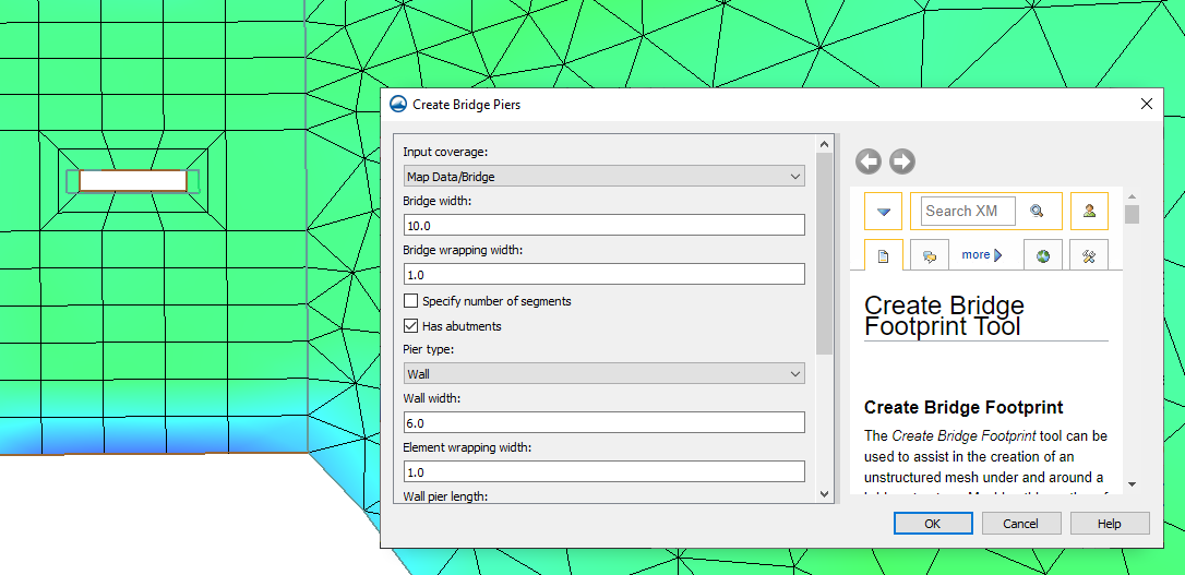
Since the real-life effects of bridges can be complex, creating a mesh to represent them is often challenging. Modeling piers and abutments using older methods in SMS requires many polygons in Mesh Generation coverages. Now, the Create Bridge Footprint tool provides an alternative approach to creating an unstructured mesh under and around a bridge structure. Note that this tool replaces the functionality made available in the Bridge-Piers coverage, which you might have been using in SMS 13.1. However, many of the same settings are incorporated in this tool as well.

The Create Bridge Footprint tool, located in the Toolbox dialog, produces a coverage and mesh that represent the bridge footprint. These features can then be used to create a mesh that incorporates the bridge footprint into the larger mesh for the model.

Example of the Create Bridge Footprint Tool

The set up for the tool includes creating a new coverage with arcs that define the new bridge:

  • The first arc should define the centerline of the bridge. It is the longest arc.
  • Other arcs, drawn across the first arc, define where the piers and abutments are located. The length of the piers is set in the tool parameters before the tool is run, so the length of these arcs is unimportant.

When drawing the feature arcs to represent the bridge for the tool, there are some important things to keep in mind. One of them is that the bridge feature arcs must be the only feature objects in the coverage. Any other objects will confuse the Create Bridge Footprint tool.

It's also important to make sure that all of the shorter arcs cross the centerline, but none of them should intersect the centerline. In this case, intersecting is different from crossing in that it creates a node on both arcs. This splits the centerline arc, making it impossible for the tool to interpret the intended meaning of the arcs.

After setting up the arcs, there are some parameters to set in the tool to complete the model of the bridge. Then the tool can be run and the resulting mesh and coverage reviewed, and you're one step closer to completing your model.

Try the Create Bridge Footprint tool in SMS 13.2 today!

Blog tags: 

Using Map from Coverage in GMS

If you are using MODFLOW 6 in GMS, you may notice that it uses a different workflow than other versions of MODFLOW in GMS. These changes were made to improve flexibility and performance for groundwater modeling in GMS. One difference is the process of mapping data from the conceptual model to the MODFLOW simulation. In all versions of MODFLOW in GMS, mapping involves taking data input in the conceptual model and "mapping" that data to the grid or mesh being used by the MODFLOW simulation. With every other version of MODFLOW, this is accomplished using the Map to MODFLOW command. However, in MODFLOW 6, mapping is accomplished using the Map from Coverage command.

Now, why this change? It mostly has to do with differences in how GMS handles these different kinds of MODFLOW. A GMS project can only hold one older MODFLOW simulation, but GMS was improved to allow multiple MODFLOW 6 simulations in a project. For handling multiple models and simulations, the Map to MODFLOW command is insufficient. There might be multiple simulations in your project, and you might not want the coverage or conceptual model you are pulling data from to map to all of these MODFLOW 6 simulations.

So how does the new command work? For a MODFLOW 6 package in GMS, do the following:

  1. Right-click on the simulation package and select the Map from Coverage command.
  2. Select a coverage for GMS to map over the package.
Example of the Map from Coverage coverage

GMS will then map the data from the coverage into the MODFLOW 6 package. It's important to note that only some of the MODFLOW 6 packages can be mapped from coverages. This means some packages must be manually set up in their package dialog. This new workflow can have some important effects on how you build your MODFLOW 6 simulation. In MODFLOW 6 it’s especially important that you map over the correct coverage. Since the data isn’t generically mapped over to MODFLOW, it’s especially necessary to know which coverage will be used to define each MODFLOW 6 package.

Try out the Map from Coverage process for MODFLOW 6 in GMS today!

Blog tags: 

Tips for Modeling 3D Bridges in SMS 13.2

Do you have an SMS 13.2 project that could benefit from using a 3D bridge? Today's blog post covers some things to consider as you model 3D bridges in SMS.

First, it’s important to know that SMS identifies the arc drawn first as the upstream side of the bridge. So the order in which the arcs are drawn affects the final bridge model. However, before the bridge is fully created, it’s possible to switch which side of the bridge is upstream using the Swap Arcs command in the Bridge dialog. Checking that the arcs are assigned to the correct side of the bridge can prevent errors later in the model.

When the bridge is created, it can be imported automatically into the model. So the bridge file is exported from SMS, but then SMS imports it automatically. To import the bridge automatically, select the Add 3D Bridge UGrid to SMS on OK option in the Bridge dialog. This eliminates the need to search for it then import it.

Example of 3D Bridge Modeling in SMS

However, if the 3D bridge file is moved, it's important to keep in mind that two files were created by modeling the bridge: an XMUGRID file and a PRJ file that contains the projection for the UGrid. These files should be kept together.

Finally, modeling piers is sometimes an important part of modeling a 3D bridge. The top and underside of a 3D bridge are defined using XY Series Editors accessible in the Bridge dialog. When defining any elevation changes in the 3D bridge, the distance (x) values cannot be identical to each other. This means it’s impossible to create a precisely vertical slope using this tool. To approximate a vertical slope, first input distance values that are very close to each other (e.g. 79 and 80). Then, pair them with elevation values that reflect the change in elevation.

Please keep in mind that piers used for an SRH-2D pressure flow model should not be modeled using the 3D bridge tool. Piers in that kind of model should be modeled using voids in the mesh.

Use these tips in creating a 3D bridge in SMS 13.2 today!

Blog tags: 

How to Export Contour Lines as Shapefiles in SMS

Have you been wanting to export the contour lines in your SMS project as a shapefile so they can be opened in a different application? SMS allows exporting contour lines as a shapefile. This post will explain how to export contour lines as shapefiles.

Saving your contours as a shapefile requires your project to be set up correctly. Save the contours as a shapefile by doing the following:

  1. Make sure the contours you want to convert to a shapefile are set to Linear in the Display Options. To do so, open Display Options and click on the page for the geometry that has the contoured dataset loaded (e.g. mesh, UGrid, etc.). First, make sure that contours are turned on. Then, click on the Contours tab. In the Contour Method in the top left, make certain the first dropdown is set to "Linear".
  2. Make sure the desired dataset is active in SMS. This can be done by clicking on the dataset in the Project Explorer.
  3. In the File menu, select the Save As command. In the Save as type drop-down menu, select Shapes Files (*.shp). Then navigate to the desired directory. Make sure it's somewhere you will know how to find it. Then click Save.
  4. Once you’ve clicked Save, a dialog opens that gives you options for converting project information to a shapefile. Select one of the contour options. The “Mesh Contours → Arc Shapefile” option is usually best.
  5. Now open your shapefile in the appropriate GIS software. The contour lines will appear as arc lines.
Example of Exporting a Shapefile from SMS

If you encounter issues with the shapefile, start by checking the folder where you saved the file. Make certain that all of the necessary files for the shapefile are there, including a projection file.

Another item to check is that everything you want in the shapefile is displayed correctly in the Graphics Window before you export. Try using the Uncheck All command in the Project Explorer and then checking only the desired geometry. This could allow you to more clearly see the contours as they will appear in the shapefile. You might also consider using the display options to turn off the geometry elements. This would also allow for clearer visualization of the contours. Once you can see the contour lines clearly, use the display options to adjust the contour lines if needed. Finally, there may be some differences between how SMS displays a shapefile and how other GIS applications display the shapefile. Opening the shapefile in SMS can help you determine if this is the case.

Be aware that selecting the Mesh Contours → Polygon Shapefile option when exporting the shapefile causes SMS to create a shapefile with only polygons. This might not accurately reflect the linear contours displayed in SMS since some of them might be only line segments.

Try out exporting contour lines as shapefiles in SMS today!

Blog tags: 

Risk Analysis for Well Groups

In your groundwater model, do you need a way to capture multiple wells for risk analysis? For example, your project might have multiple pumping wells and you would like to see the probabilistic composite capture zone for all wells in the wellfield. GMS provides a way to access the Risk Analysis dialog for refining stochastic modeling results.

Example of the Risk Analysis Wizard in GMS
  1. First open your project in GMS, making sure to select the Plan View and 3D grid module, it will be more difficult to select wells otherwise.
  2. Using the Select Cells tool, drag a box around the entire grid to select all cells in the grid.
  3. Open the 3D Grid Cell Properties dialog and change the value for the MODPATH zone code to a number of your choice.
  4. Select the coverage of the well to make it active. Using the Select Points/Nodes tool, drag a box around the entire project to select all wells in the coverage.
  5. Select Intersecting Objects to open the Select Objects of Type dialog.
  6. Select 3D grid cells from the list and close the dialog. This will select all 3D grid cells that have a well in them.
  7. Open the 3D Grid Cell Properties dialog.
  8. Change the value for the MODPATH zone code to a different number than the one that was used before, close the dialog and save changes. From here, the probabilistic capture zone analysis should be able to run with the well groups setting turned on.

Please note that particles need to leave their original zone to be mapped on the risk analysis results. That is why nothing will show up when all cells were assigned to the same zone. The recommended solution is to change the zone code of just the cells with a well so that as many particles as possible can leave the assigned area.

GMS allows you to be as general or specific as you need when selecting wells for risk analysis. Try out using risk analysis for well groups using GMS today!

Blog tags: