Using MODFLOW-NWT for Mine Dewatering
By aquaveo on July 22, 2020Have you tried dewatering a mine model using MODFLOW-NWT? MODFLOW-NWT is a version of MODFLOW provided by the USGS that uses a method to solve MODFLOW models that are non-linear due to unconfined cells or non-linear boundary conditions, creating an asymmetric results matrix. Because mines that need to be dewatered sit below the water table, cells within the simulation will become dry at times due to the removal of the water from the mine. MODFLOW-NWT is great for such situations as it handles dry cells well.
Mine dewatering models are often used when estimating the required flow capacity for the pumps used in the field. You can create a regional model to establish a baseline, then create one or more models with various pit depths to establish the best approach for the mine in question. While elevations cannot be set to transition during a MODFLOW run, multiple conceptual models can be created within the same project in order to keep all of the data together.
It’s important to remember the difference between wells and drains when creating the dewatering model. Drains only subtract water when the head is above the elevation of the drain. Therefore, drains can be used to represent the seepage face around the edges of the pit, and the drain elevations should be set to equal the ground surface elevations. The amount of water removed by a drain is related to the conductance of the material of the seepage face. Drains are generally used at the bottom and side seepage faces of the mine.
Wells remove a specific amount of flow, and can therefore dewater the cell they are in prior to dewatering the rest of the mine. MODFLOW-NWT, as mentioned previously, handles these dry cells very well, keeping them active in case they become wet again.
Because MODFLOW-NWT uses 3D grids, you should make sure the cells inside the pits are inactive. You do this by creating the boundary polygon, and then removing a "donut hole" of cells within the pit area. Use the Activate Cell(s) in Coverages tool to inactivate the cells. You’ll have to do this for each layer, and each layer should be on its own coverage.
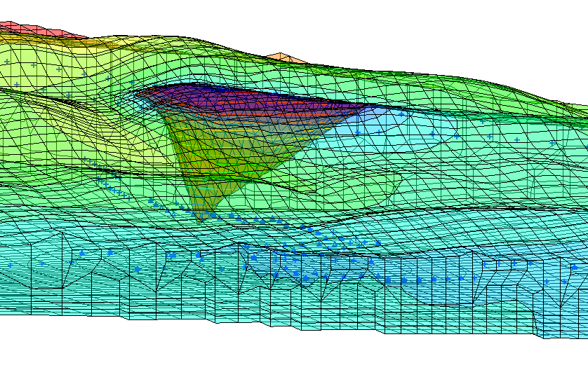
Finally, always use the Model Check to make sure there aren't any obvious errors or missing values in any of the inputs. After MODFLOW-NWT finishes running, you should review the water table by looking at the drawdown output contours. You can also do this by switching to Ortho view and reviewing the head in the appropriate rows or columns.
Try out making a mine dewatering model using MODFLOW-NWT in GMS today!