Introducing HydroGeoSphere with GMS
By aquaveo on January 23, 2024The Ground-water Modeling System (GMS) 10.8 beta includes a model interface that is brand new to the software. HydroGeoSphere (HGS) is a unique three-dimensional control-volume finite element simulator developed by Aquanty that is meant to be able to handle all parts of the terrestrial water cycle. It uses a globally-implicit approach to simultaneously solve the 2D diffusive-wave equation for overland/surface water flow and the 3D form of Richards’ equation for variably saturated groundwater flow. This is different from the many other models that simulate only a portion of the hydrologic cycle. HGS includes components for precipitation, evaporation, overland flow, infiltration, recharge, and more. HGS can simulate both surface and subsurface water flow simultaneously for each time step.
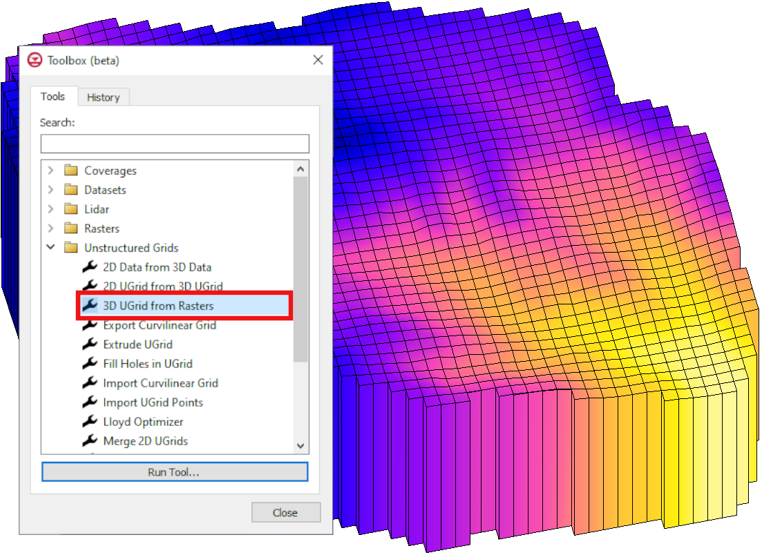
In GMS, the base components for an HGS model include: an unstructured (UGrid), HGS coverages, and an HGS simulation. GMS allows multiple HGS simulations to exist in a single GMS project. A 3D UGrid of the project area is required before building an HGS simulation. There can also be multiple UGrids in one project, although only one UGrid can be assigned to each simulation.
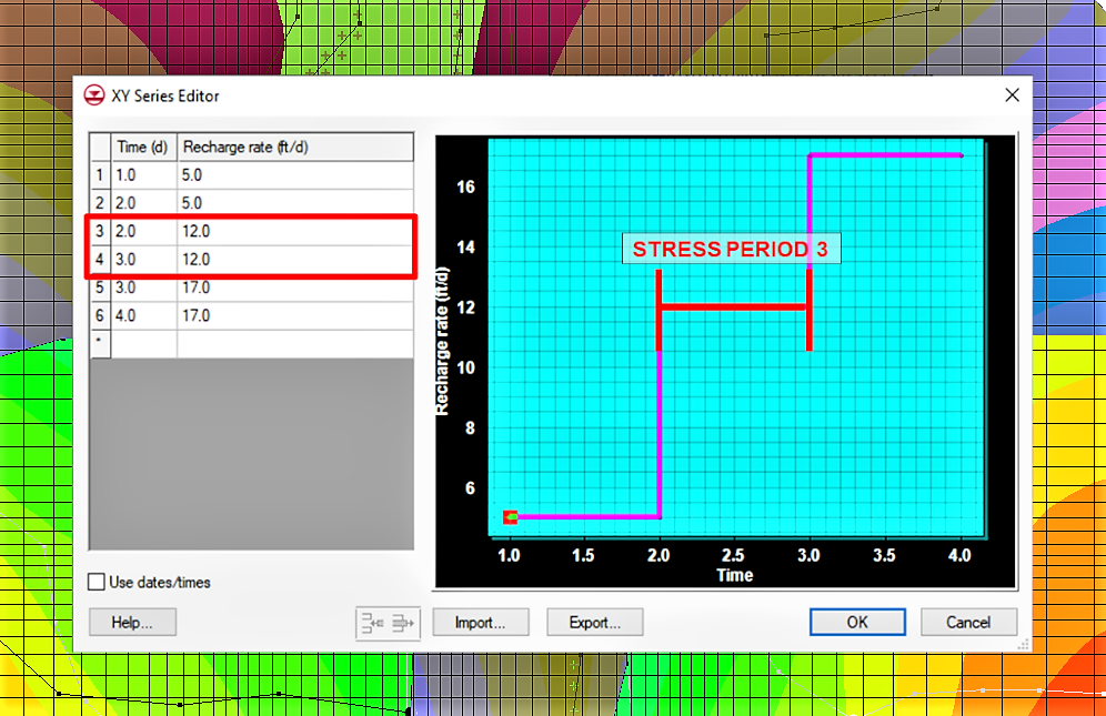
The coverages specific to HGS are boundary conditions, observations, and hydrographs. GMS uses feature objects to define the boundary conditions on an HGS boundary conditions coverage. This includes points, arcs, and polygons. The observations coverage allows you to set observation points that will collect time series information during the simulation run. The hydrograph coverage records hydrograph data during the simulation run.
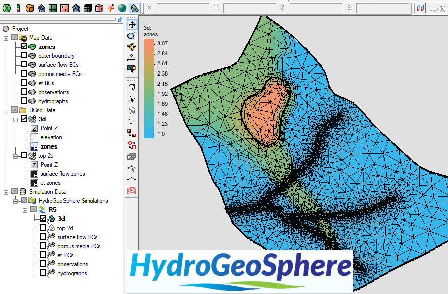
HGS defines materials with domains and zones. The domain contains information about the type of material. The domain is then assigned a zone number, which is then assigned to a polygon. Multiple domains can be assigned to the same zone.
There’s a lot more to HydroGeoSphere than we can cover in one blog post. If you’d like to learn more about HGS, Aquanty has numerous resources on their website. You can look at the HGS Theory Manual or the HGS Reference Manual. They regularly post webinars on their blog and on their LinkedIn. You can also find videos about how to use HydroGeoSphere as well as presentations that have been made by Aquanty’s staff on their YouTube page. We also have our own HGS tutorials that can walk you through the steps of building an HGS model.
We hope you’re excited about the addition of HydroGeoSphere into GMS 10.8, because we certainly are! Download GMS 10.8 to try out HGS today!
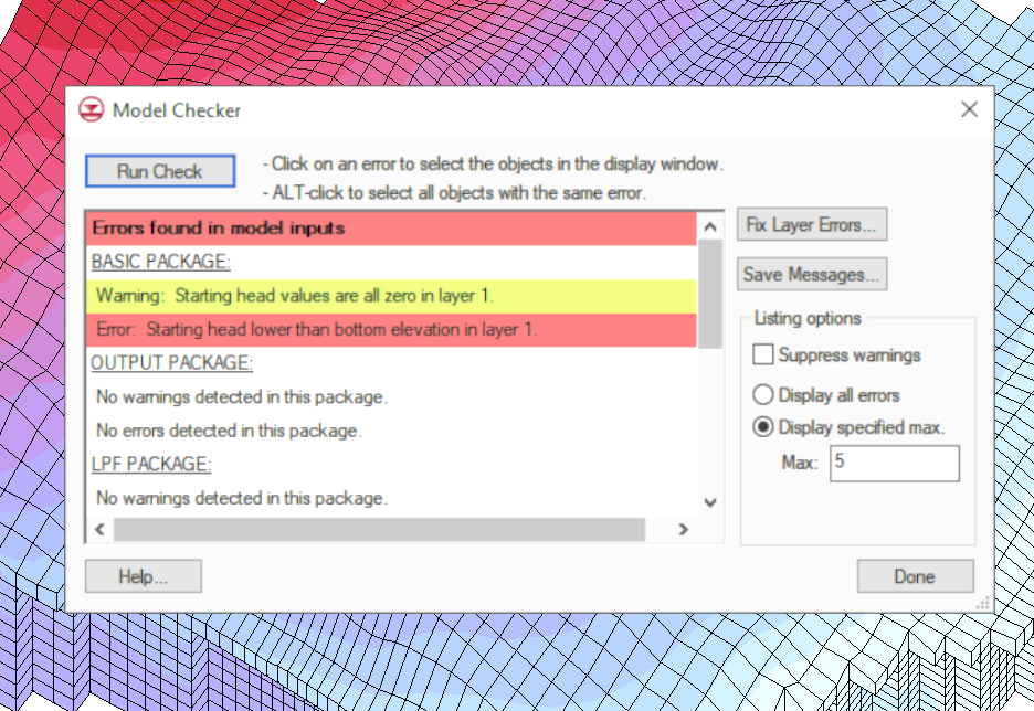
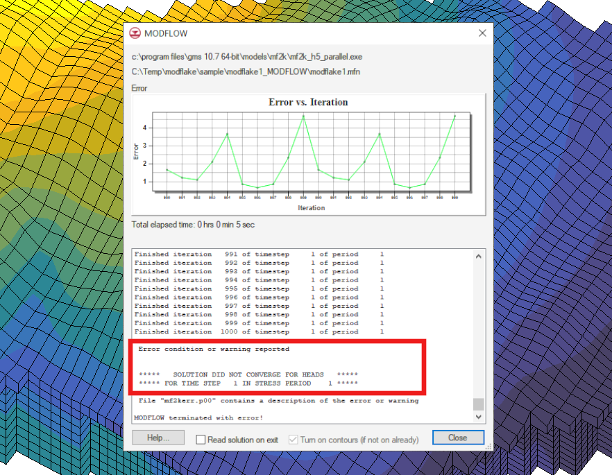 The next thing to look at in your MODFLOW model when you’re trying to figure out what the issue may be is the command line output from the