Draping an Image onto a Ground Surface
By aquaveo on May 24, 2018When looking at your GMS project in oblique view or when using the Rotate tool, you might have noticed that your map image will disappear. This is because GMS only supports viewing map images in plan view. However, there is a way to make the map image visible in these views.
The ability to drape an image in GMS has been around since the early versions. However, you may not have had an opportunity to use it, or you simply missed hearing about it among all the other great things GMS does.
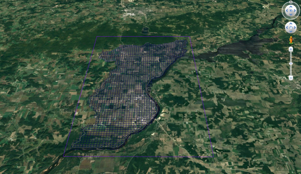
When not in plan view, an image can be draped on the top surface of a TIN, mesh, or grid. When this is done, the map image will remain visible even when rotating the display view. Some relationships between the surface texture and the shape of the terrain can become visible after the image has been draped over the terrain surface.
If you didn’t already know how to drape an image in GMS, or you want a refresher on how to do it, this is what you do:
- Turn off Ortho Mode if it is active. Draping an image cannot be done using Ortho Mode.
- Select and make active the map image you want to view. You can use any image file type that GMS can import.
- Select a dataset under your grid, mesh, or TIN in the Project Explorer and make it active. A draped image is only applied to one dataset at a time.
- Open the Display Options dialog.
- Select the appropriate grid, mesh, or TIN display tab.
- Turn on the Texture map image option.
- Use the Rotate tool or any of the view options to see how the image mapped to the top surface of the geometry.
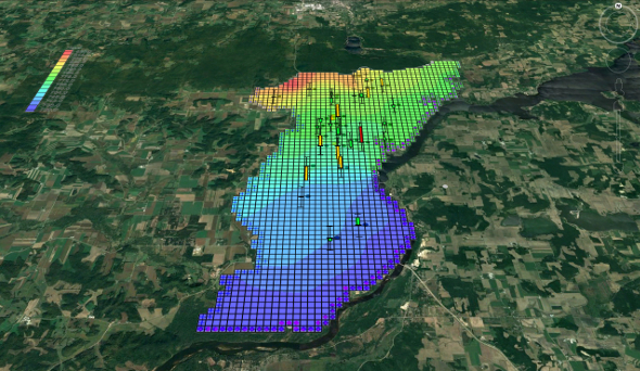
Here’s an example of how it will appear:
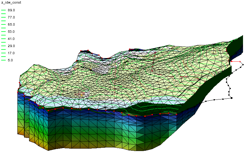
If desired, you can adjust the Lighting Options in GMS to make the features smoother or sharper.
Now that we’ve reviewed the steps, try draping images in GMS today using the GMS Community Edition.