Aquaveo & Water Resources Engineering News

Creating a Pathline for Every Time Step With MODPATH

Have you ever wanted to be able to visualize the movement of particles along every time step in a MODFLOW simulation using MODPATH? MODPATH is a program in the Ground-water Modeling System (GMS) for tracing particles that is utilized in conjunction with the flow data in a MODFLOW simulation. MODFLOW defaults to showing particle movement one time step at a time, but it is possible to show all time steps at once by making use of the Pathlines → Arcs feature.

Example of pathlines generated by MODPATH

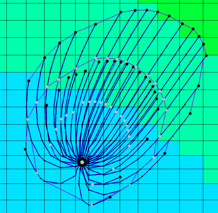
To create the particle pathlines as arcs, you need a complete MODFLOW and MODPATH simulation. Once you have that, creating arcs to represent every time step is as simple as going to the MODPATH menu and selecting Pathlines → Arcs. This will create new coverages under your Map Data, the number of which will depend on how many Particle Sets exist in the simulation. It may be useful to go to your display settings and make sure that vertices are turned on under Map Data to see the time steps along the pathline arc more clearly. Each segment of the arc represents a single time step, with the subsequent segment starting where the previous ended.

By right-clicking on one of the particle sets, you can select View Pathline Report, which will show the same data from the arcs on a table. By doing this, you can view the exact values for each point and vertex along the pathline arc. You can also export this data as a text file, which can be opened in Excel in order to view the data outside of GMS. Additionally, you can view the data in several different types of plots by using the Plot Wizard under the Display menu.

You can also export the data from each particle set as a shapefile, making it simple to import the pathline arc data into a different project or program. To do this, all you need to do is right-click on the particle set, export the data, and save it as a Pathline Point Shapefile (*shp).

Head over to GMS and try out the different ways to visualize particle data with MODPATH and MODFLOW today!

Blog tags: 

Filling Missing Raster Data

Do you have a raster that has holes in it? The Fill Nodata can fix small holes in raster data. Available in GMS, SMS, and WMS. In this article, we will explore the ways that the Fill Nodata tool can be used in WMS.

The Fill Nodata tool fills in small areas or gaps in a raster where no elevation data exists. It is located in the Rasters/Fill Nodata section of the Toolbox. The tool will interpolate an elevation to raster cells that are classified as "NODATA". Then the tool will create a new raster in the project that has the fillable no data areas filled.

Example of the File Nodata tool

These holes in the raster can occur for a number of reasons, one of the most common being that the data is incomplete. WMS is flexible enough that it can use a raster with small amounts of missing data for most simulations. However, it is recommended that you have data that is as complete as possible to ensure the generated model is as accurate. Therefore using the Fill Nodata tool can help ensure the accuracy of your model.

The Fill Nodata tool has a few input parameters to keep in mind. The input raster is the most important parameter. This needs to be a raster that has been imported into the project. The maximum distance to interpolate determines how far out WMS will look to fill data. It will use pixel units to do this. The number of 3x3 average filter smoothing iterations to run determines how many smoothing interactions will be run after the interpolation has been calculated. Additional interactions can help in improving the fill data.

Keep in mind that the tool was not intended to create data for large regions of missing data cells, especially regions on the border of the raster. If you have a large area of missing data, it would be best to use other processes to fill in the missing data, such as downloading the missing data and merging it with your raster.

The Fill Nodata tool is one of thetools provided in WMS to let you modify and edit raster data. Try out the Fill Nodata tool in WMS today!

Blog tags: 

Converting a 2D Mesh to a CAD Surface

Using CAD files can be a useful way to transfer project data between different modeling software that may not support all of the same file types. The Surface-water Modeling System (SMS) supports the conversion of terrain in the form of scatter surfaces and mesh surfaces to and from CAD data for easy transfer between systems that utilize CAD data.

To save a terrain from SMS as a CAD surface file:

  1. Deselect everything in the Project Explorer that doesn't contain the terrain data you want to work with. Depending on the amount of data currently in the Project Explorer, the simplest way to achieve this may be to right-click on an empty section of the Project Explorer and select "Uncheck All".
  2. Reselect the terrain data in the Project Explorer.
  3. Right-click in any empty space in the Project Explorer and select "Save as CAD". A save window will pop up and you'll be able to name the CAD surface file and choose where it will save outside of SMS.

The CAD surface data will then also appear in the Project Explorer. Once you assign a name to the file, you should be able to import it into your CAD software and make modifications. This file set will contain all the necessary surface data, including elevation, node, and element information.

Using CAD Faces to 2D Scatter Triangles

When importing CAD surface data into SMS, you'll need to convert it into a form that SMS can recognize so you can make changes and use the information stored in the file. To convert the data back into a form you can use within SMS, you just need to right-click on the CAD data under the CAD Data file folder in the project explorer. Then, select the "Convert → CAD Faces → 2D Scatter Triangles" command.

Head over to SMS and see how using CAD data can benefit your project today!

Blog tags: 

Converting a 3D UGrid in GMS

Have you ever had an unstructured grid (UGrid) or mesh in your project in the Groundwater Modeling System (GMS) that you want to convert to another geometry? While there isn't a specific tool for converting UGrids in GMS, it can still be achieved by following a few simple steps. Typically a UGrid will need to be converted to a scatter set and from there the scatter set can be converted to other geometries. Converting UGrids or mesh into scatter points can be a good way to compare data between models, especially if one of the models is older and doesn't, or can't, include a UGrid or mesh. If this is something that interests you, this article will explain how to get from a UGrid or mesh to either 2D or 3D scatter points.

Example of converting a scatter set

First, go to the Display menu above the macros in the GMS window. Then choose Convert to CAD. Note: CAD data. is generated from whatever is currently visible in the Graphics window, so make sure that everything you need is displayed before you continue. The new CAD data will appear in the project window as a (*.dwg) file. Now right-click on the CAD data and convert CAD Points to TIN Points. A dialog window will appear asking you to designate which layers of the data you want to include in the conversion and to name the new TIN. You can customize this in whichever way best suits your needs.

This new TIN data can be converted directly into a scatter set. Right-click on the TIN and convert it into a 2D scatter set. 3D scatter sets can be made by simply executing a conversion one more time with the 2D scatter set.

If ultimately you want to compare scatter data with another model, it may be helpful to be able to view both sets of data in the same window. You can easily export the scatter set from GMS by right-clicking on the scatter set in the project window and selecting Export, then open the newly exported file in the GMS window with your other project. The scatter set can also be used to create a boundary for a 2D or 3D Cartesian grid which could be used with an older version of MODFLOW.

Head over to GMS and try converting UGrids into scatter sets today!

Blog tags: 

Working with ADCIRC Levees in SMS

As a oceanic modeler working with hydrodynamic modeling, you may have an ADCIRC levee structure in your project that you need to check or fix. Fortunately, SMS provides a couple of tools that can assist you with this task. These tools are part of the SMS Toolbox and allow you to test and verify that levees are working properly. In this article, we'll take a closer look at these tools and how they can be used to enhance your surface-water projects.

To access the ADCIRC levee tools, you can open the Toolbox and expand the ADCIRC folder. The first tool available is called Fix Levee Crest Elevations. This tool checks the ADCIRC boundary conditions coverage that contains the levee arcs. It compares the Z crest attributes against a set of elevation lines, which are known as check lines. The tool will perform a check on any selected levee arc or all levee arcs if none of them have been selected previously. If the elevation values are outside of the check lines, the tool will adjust them to fix the values.

Another tool in the toolbox is the Check/Fix Levee Ground Elevations. This tool checks the elevations of an ADCIRC domain based on the crest elevations defined in an ADCIRC boundary conditions coverage. If necessary, the tool will lower the elevations of a domain based on the elevations defined in the boundary condition coverage. This tool also creates a new dataset that can be mapped as an elevation for the 2D mesh if desired.

Example of the Check/Fix Levee Ground Elevations tool

Both of these tools check the validity of the levee. If the levee does not line up with a hole in the mesh, the tool will determine it to be invalid. If the tool determines the levee to be valid, it will run, and the output datasets will be loaded onto the input domain mesh in SMS.

The ADCIRC levee tools are just some of the tools available in the SMS Toolbox. Additional tools will be added in the future to enhance the capabilities of the toolbox. By using the Toolbox for your surface-water projects in SMS, you can easily test and verify the effectiveness of levees and ensure that they are functioning as they should be.

In conclusion, if you need to check or fix an ADCIRC levee structure in your project, SMS provides helpful tools in its toolbox to assist you. These tools, such as Fix Levee Crest Elevations and Check/Fix Levee Ground Elevations, allow you to test and verify the effectiveness of levees, ensuring that they function correctly. So, try out the SMS toolbox today for your surface-water projects, and make your work easier!

Blog tags: 

How to Include Sediment Transport in CMS-Flow

As a civil engineer working with hydrodynamic modeling, you understand the importance of considering sediment transport in many models, such as CMS-Flow. The sediment transport equation is essential as it models the rate of sediment particle movement based on various factors, including local flow conditions and sediment properties. With the sediment transport module in CMS-Flow, you can achieve a more accurate representation of river or coastal systems. It also enables you to explore different scenarios such as changes in flow conditions, sediment input, or sea level rise.

Using the Surface-water Modeling System (SMS), the base of a CMS-Flow model is created on an unstructured grid (UGrid), with components such as save points, activity classification coverage, and boundary conditions. Save points are vital for identifying high temporal resolution output locations. Activity classification coverages exclude geographic regions from the simulation computations. A boundary conditions coverage is a required component for any simulation.

Example of Sediment Transport options for CMS-Flow

Once you have created these components, you can create a new CMS-Flow simulation by right-clicking in the Project Explorer. Next, apply the UGrid and any coverages you want to include in the simulation by dragging them under the simulation. You can then set the parameters for sediment transport by following these steps:

  1. Right-click on the simulation and select Model Control to open the CMS-Flow Model Control dialog.
  2. Select the Sediment Transport tab and check the box next to Calculate sediment transport.
  3. Under the Sediment Transport tab, input various parameters to refine sediment transport in the simulation. These include sediment density and porosity, bed composition, transport formula, and more.
  4. Set all other desired parameters in the tabs of the CMS-Flow Model Control dialog and click OK when finished.

Once you have set all the necessary parameters, you are ready to run the CMS-Flow simulation with its included sediment transport calculations. By utilizing sediment transport, you can refine your CMS-Flow model further and achieve more accurate results.

In conclusion, sediment transport is an essential process that needs to be considered in hydrodynamic models like CMS-Flow. With the sediment transport module in CMS-Flow, you can achieve a more realistic representation of river or coastal systems and explore various scenarios. Follow the steps outlined above to set the sediment transport parameters and refine your CMS-Flow model in SMS today.

Blog tags: 

Exploring the MODFLOW HUF Package

Are you looking to control flow between grid cells in your MODFLOW project using the Ground-water Modeling System (GMS)? MODFLOW offers a couple packages for doing this, but consider using the Hydrogeologic-Unit Flow (HUF) package. This package gives you greater control over the properties of cells regulating flow in a MODFLOW model and help represent more complex stratigraphy in your project.

The HUF package is located in the MODFLOW Global options, and can be used in conjunction with other packages. The HUF package is one of the flow packages, of which you can only have one flow package selected for a project. Once the HUF package has been added to the project, it can be accessed through the MODFLOW menu.

Example of HUF package materials

The benefit of using the HUF package in your MODFLOW model is that the materials are not bound to the grid, making it possible for there to be more than one material mapped to a single cell. The hydrogeologic units are calculated independent of the cell boundaries, so by using the HUF package the model can more accurately represent the relationship between materials.

View the hydrogeologic units by going to the display options and clicking on the MODFLOW tab under 3D Grid Data, then turn on Hydrogeologic units. Back in the Graphics Window, when in ortho mode, you can view the model from the top, front, or side.

By accessing the HUF package under the MODFLOW menu, you can select the Edit Materials button to view or change the conductivity level of each material. In the HUF package dialog, you can also edit the top values or thickness values in the array manually, and designate whether to use vertical hydraulic conductivity (VK) or vertical anisotropy (VANI). You can also define each layer as confined or convertible, assign a head to dry cells, adjust grid elevations, and more. The HUF arrays can also be exported to grid datasets, which makes them viewable as contours or in a table.

Incorporating the HUF package into GMS also expands how the package can be used. For example, GMS has the ability to use TPROGS to generate HUF data.

Go to GMS and see how the HUF package can be used in your MODFLOW model today!

Blog tags: 

Using CAD Data to Delineate a Watershed

Did you know that you can use CAD files to delineate your watershed area in a Watershed Modeling System (WMS) project? WMS is capable of using CAD data for elevation data, designs, layouts, and more. CAD data can be converted to TINs and feature objects to be implemented in a WMS project.

When converting the CAD data to feature objects, you can choose which layers from the data you would like to use when creating the new feature object. After that, you can clean up the feature object and choose all the properties for the coverage. To convert CAD data into feature objects, do the following:

  1. Import the CAD data into WMS from a DWG, DXF, or DGN file.
  2. After importing the CAD data, review the data to verify that it was imported correctly and that it has the correct projection.
  3. Right-click on the file in the Project Explorer and select Convert | Feature Objects….
  4. In the Cad → Feature Objects dialog, select which layers to convert into feature objects.
  5. Make certain the new coverage is set to have the "drainage" type.
  6. Designate the converted feature objects as outlet points and streams. Also verify that any stream arcs a set with the correct direction.

With the CAD data converted to feature objects and you've designated your outlets and streams, you can start the process of delineating your watershed. To do this, you will need a DEM in your project. If you have elevation data stored in a CAD file, you will first need to convert the CAD data to a TIN.

Basin delineated from CAD data

CAD data can be converted into TIN points or TIN triangles, but the best way to end up with TIN triangles is to convert into TIN points first. To convert CAD data directly into TINs, do the following:

  1. Import the CAD data into WMS in the form of a DWG, DXF, or DGN file.
  2. Right-click on the file in the Project Explorer and select Convert | CAD Points → TIN Points.
  3. In the Cad → TIN dialog, select which layers to convert and the name the TIN data will appear under in the Project Explorer.
  4. Right-click on the TIN point data in the Project Explorer and select Triangles | Triangulate.

From here you can convert the TIN to DEM if necessary. The TIN module in WMS has a few tools for working with basins that may be sufficient for your model. However, some models either perform better or require a DEM. Once you have the DEM you can generate the delineated basin. To do this:

  1. Right-click on the TIN and select Convert | TIN → DEM.
  2. Enter parameters for the DEM in the Convert TIN to DEM dialog.
  3. Review the generated DEM.

Once you have a DEM, complete the following steps:

  1. Select DEM | Compute Flow Direction in the Drainage module.
  2. Select DEM | Polygon Basin IDs →> DEM in the Drainage module.
  3. Select DEM | Compute Basin Data in the Drainage module.

Once you have a delineated basin, you can use the basin with the watershed modeling model of your choice. Be certain to review the basin to make certain it contains all of the area you need for your project.

Head over to WMS and see how you can utilize CAD data to create delineated basins in your projects today!

>
Blog tags: 

Methods for Redistributing Vertices

The ability to redistribute vertices along an arc can be essential for any number of projects. The Surface-water Modeling System (SMS) offers a couple of different methods for redistributing vertices. This post will examine two of those methods.

The Redistribute Vertices Dialog

The first way to redistribute vertices is relatively simple. Select an arc, or multiple arcs, and either right-click and select Redistribute Vertices from the menu, or go to the Feature Objects menu and select the Redistribute Vertices command. This will pull up the Redistribute Vertices dialog window. From there you have a few different options as to the method of distribution.

  • Specified spacing: the number of vertices on an arc will be determined by how far apart the vertices should be.
  • Number of segments: how many pieces the arc should be broken up into.
  • Min/max spacing: with min/max spacing, the segments will start at the minimum set length and gradually get longer until the last one is the maximum set length.
  • Source arc: this requires you to choose two arcs. The number of vertices on the target arc will change to match the source arc.
  • Size function: this option requires a data source.
Example of the Redistribute Vertices dialog in SMS

In the Redistribute Vertices dialog you can choose to include a bias with specified spacing and number of segments options. Using a bias means that each segment will be a percentage larger or smaller than the one before it, which depends on whether or not the bias number is less or greater than one. The direction of the bias is determined by the direction in which the arc was created. For example, an arc created top to bottom will have the smallest segment at the top and the largest at the bottom if the bias number is greater than one.

The 2D Mesh Polygon Properties Dialog

Another option available in SMS is to use the 2D Mesh Polygon Properties dialog when redistributing vertices along the arcs of a polygon. This can be used on any polygon that has been created on a coverage. There are three ways to access the 2D Mesh Polygon Properties dialog window, but the simplest option is to double-click on the polygon itself.

Example of redistributing vertices with the 2D Mesh Polygon Properties dialog in SMS

The 2D Mesh Polygon Properties dialog window is primarily used for creating a mesh inside a polygon. However it can still be used to redistribute the vertices along an arc. The benefit of using the 2D Mesh Polygon Properties dialog window rather than Redistribute Vertices is that it offers a preview option so you can see what the polygon will look like with the new vertex distribution without having to open and close the Redistribute Vertices dialog to see the changes. This makes it easy to test out different options right in the same window. The downside of using this dialog window rather than Redistribute Vertices is that it doesn’t offer the same range of redistribution options. The only redistribution options the 2D Mesh Polygon Properties dialog offers for vertices is specified distribution along the arc, with or without a bias. If you’re looking for more specificity, this may not be the right option for your project.

Try the different methods of redistributing vertices in the SMS today!

Blog tags: 

Setting Up a Cross Section Animation in GMS

Have you ever wanted a way to better visualize cross sections in your project? The Animation Wizard in the Ground-water Modeling System (GMS) can help you do just that. Any project involving a 3D mesh or 3D grid can utilize the cross section animation feature.

To build your initial cross section, you’ll need to start with a 3D mesh or grid as a foundation. After your foundation is set, build the cross section. Keep in mind that the Animation Wizard will create the animation through what is currently visible in the Graphics Window, so it is a good idea to get the display settings where you want them before starting the animation process.

Go to the Display menu and scroll down to the bottom to find the Animate option. Before initiating the animation, make sure that the cross section is active in the Graphics Window. Note that although the cross section needs to be active to create the animation, it doesn’t need to be turned on if you don’t want the static cross section from the project to be visible.

Example of the setting up a cross section animation in GMS

In the Animation Wizard dialog, turn on Cross-sections/Isosurfaces under Steady State. This is the option that animates the cross sections. You can change the speed of the animation by altering the number of frames per second, which is on the first page of the Animation Wizard, and the number of frames, which is on the second page. The lower the number of frames per second, the longer the animation will spend on each cross section, and vice versa.

The second page of the Animation Wizard is where you can specify the plane over which the cross sections will be animated. You can animate over the X, Y, or Z-axis, or any combination of the three. You can also alter more of the display options for the animation under the Cross Section Option button on this page.

After clicking Finish, the Animation Wizard will automatically export the cross section animation as an MP4 file, and you can open the MP4 file to view the finished product.

Even more settings and options are available that were not covered in this post, explore what cross section animations can do for your GMS project today!

Blog tags: 

Pages