Aquaveo & Water Resources Engineering News

How to Turn on Hydrographs for GSSHA Outlets

Are you needing to enable hydrographs in your GSSHA model in the Watershed Modeling System (WMS)? Hydrographs are a valuable tool included in WMS for understanding water dynamics in your model. In this blog post, we will learn about the process of enabling them within your GSSHA model.

The Gridded Surface Subsurface Hydrologic Analysis (GSSHA) model is a two-dimensional finite difference rainfall/runoff model. GSSHA uses a grid to establish the computational domain and parameters for surface runoff. The GSSHA model is fully coupled with hydraulic stream flow/routing models. After building a GSSHA model in WMS, you can create hydrographs to analyze the results.

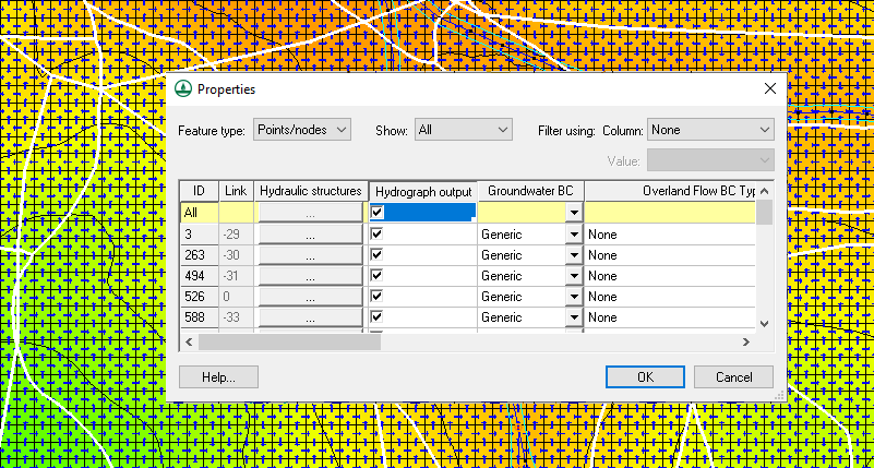
Select a Sub-Basin Outlet Point within your GSSHA model, and identify one of the points where you want to monitor water flow and drainage closely. When using a GSSHA type coverage, the hydrographs can be turned on or off in the point attributes dialog. To access this dialog:

  1. Select one of the sub-basin outlet points, and right-click it and choose Attributes.
  2. In the Properties dialog that appears, turn on the checkbox labeled Hydrograph Output.
  3. Click out and this will turn on the hydrograph for that particular point.
  4. Next, re-run GSSHA. This is a crucial step because new GSSHA results will be needed to access the hydrograph.
Example of Hydrograph for GSSHA

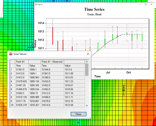
After the new solution is loaded, you should see the hydrograph icon next to that point. From there, you can select and view it. Now, you can read the data and gain valuable insights into water flow dynamics at that location.

It is important to note that if you do not see the hydrograph icon then it is likely that WMS did not register you turning on the hydrograph option for the location. Check the properties for the model to see if the hydrograph output options were correctly saved.

Turning on Hydrographs for different outlets is one of the many options you can use with GSSHA in WMS. Try out turning on Hydrographs for different outlets and other options for GSSHA in WMS today!

Blog tags: 

Using the Hydraulic Toolbox with SMS

You may have already used the Hydraulic Toolbox to define a culvert for an SRH-2D model, but did you know its suite of calculators can assist you in many ways when creating a simulation in the Surface-water Modeling System (SMS)? The Hydraulic Toolbox is a software developed for the FHWA by Aquaveo, and there are many uses for the calculators, but today we’ll go over one example today to give you an idea of what you can do.

The Hydraulic Toolbox can assist you with calculations for other simulations, such as an SHR-2D urban hydraulics project in SMS. One of the main calculators that can be used for urban modeling with SRH-2D is the Curb and Gutter flow analysis.This calculator examines flow across storm drain inlets for various curb and gutter openings.

Example of the Hydraulic Toolbox with SMS

The Hydraulic Toolbox includes a macro that opens the Curb and Gutter Analysis calculator, or you can access it through the Calculators menu at the top of the window. This adds it to the Project Explorer under a “Project” folder. Once it has been added to the Project Explorer, double-click on the tool to open the calculator’s dialog. There are three main parts to the calculator: Gutter, Inlet, and a Parameters table. The Gutter section contains values for the gutter dimensions. This includes, but is not limited to, the gutter width, design flow, width of spread, etc.. The Inlet section is where factors defining the inlet location, inlet type, grate type, etc. are included. The Parameters table displays all the inlet data after it has been calculated by using the “Compute Inlet Data” button.

The Hydraulic Toolbox is separate from SMS, so as of SMS 13.3, data from the calculator will need to be entered manually into the relevant portions of SMS. The calculated data can easily be viewed from the calculator dialog itself, or you can export a document that contains a list of all of the data from the calculator. The Create Report function can be performed by right-clicking on the project folder in the Project Explorer, clicking the “Create Report” macro, or finding the Create Report option under the Calculators menu.

You can also attach notes to the project in the Hydraulic Toolbox. The options that allow you to create notes are found in the same three locations as the Create Report function, detailed above.

More in depth information about how the Curb and Gutter calculator, as well as the Hydraulic Toolbox in general, works can be found in the User’s Manual, which is accessed through the Help menu in the Hydraulic Toolbox. The Hydraulic Toolbox can be downloaded from this link.

The Curb and Gutter analysis calculator is just one example of how you can use the Hydraulic Toolbox with SMS. Head over to SMS and the Hydraulic Toolbox to explore the variety of calculators and how they can help you with your project today!

Blog tags: 

How to Refine an Unstructured Grid

When working with a multi-layer unstructured grid (UGrid) in the Ground-water Modeling System (GMS), your project may require different levels of refinement in each layer to introduce complexity to the stratigraphy. GMS currently offers a limited number of ways to achieve this in a 3D UGrid module. Mapping coverage directly to a 3D grid simplifies vertical refinement considerably, but it results in all layers being of uniform size. This blog post will cover the most straightforward way to create a complex stratigraphy, as well as some things that may be useful to know about how refining grids works and what the limitations are.

The type of grid that will often get you the closest to where you want to be is a Quadtree grid. These are the steps you’ll want to follow:

Using the Refine command to refine a quadtree
  1. Use the TINs/Horizons to UGrid approach to generate a grid that incorporates the desired pinchouts and ensures an appropriate level of refinement for the least refined layer.
  2. Right-click on the Quadtree UGrid in the Project Explorer and scroll to the bottom of the UGrid Properties dialog window.
  3. Make sure the Constraint dropdown is set to "None". If the constraint is set to "3D", you will not be able to refine the UGrid cells.
  4. Note that you can’t change the constraint back to "3D" after changing to "None", so you may want to duplicate the UGrid and make changes to that one to preserve the original.
  5. In the toolbar above the Graphics Window, check the box for Single Layer to isolate a layer of the grid for refinement. Highlight the cells you wish to refine using the Select Cells tool.
  6. Right-click on the selected cells and choose Refine.

The newly generated UGrid maintains the original level of refinement on all layers except for the one where you just refined some of the cells. You can repeat this process as many times as needed to achieve the desired level of refinement.

Currently, there is no automated process for this kind of complex refinement, so while it is possible to use this process on a larger project, it may not be practical. If you have a limited number of areas to work on, this workflow lets you produce a grid that features your desired TIN pinchouts, with varying levels of refinement for different layers. It is also not possible to un-refine a grid, so you’ll always need to start with the least refined layer and work your way to the most refined.

Head over to GMS and try this method to refine your 3D grid today!

Blog tags: 

Tips for Locating the Correct Projection

It is crucial that data brought into GMS, SMS, or WMS contain the correct coordinate system. The coordinate systems are designated through the use of projections. But what do you do if you import data and it doesn’t have the correct projection information or is missing projection information all together?

Example of The Display Projections dialog

If you know what projection the data is supposed to be set to, use either the Display Projection dialog to set the projection for the project or right-click on the data in the Project Explorer to set the object projection. It is recommended that all data in a project use the same projection. To set the projection using the Projection dialog, do the following:

  1. Go to the Display menu at the top of the window and select Display Projection. This will bring up the Display Projection dialog.
  2. Under the Horizontal section, if “No projection” is selected, change it to “Global projection”. If “Global projection” is already selected and you want to change the projection, select the Set Projection… button.
  3. /From the dialog that opens, you can search through the provided database for the correct projection, or you can import a projection (*.prj) file from outside the application.

More information about the Display Projection dialog can be found here [2]. The object projection is set through the Project Explorer right-click menus, but otherwise follows a similar workflow.

If you already have data imported into the project that has the correct projection, see if you can reproject the data with the incorrect or missing projection. In general, you can reproject the data by right-clicking on a specific data object in the Project Explorer. With SMS, you can also go to the Display menu at the top of the window and select Reproject All… to reproject the data all at once.

If you don’t have a projection, use the Online Maps tool to locate the correct area in the world, then download the data using Online Maps to obtain coordinate data. Set your data to use this projection. Make certain the data lines up correctly with the downloaded data.

Rarely, the project information is included in the data but XMS fails to read the projection. This is often the result of a formatting issue. Try opening the file in a text editor to see what projection information is there. Then either adjust the formatting so XMS can read the projection information, or set the projection for the data after importing.

Head over to any of the XMS products and see how projections work today!

Blog tags: 

Using SRH-2D Initial Conditions

Are you wondering which initial hydraulic condition to use for your SRH-2D model in the Surface-water Modeling System (SMS)? Setting the initial condition for how each cell is to be treated in an SRH-2D simulation is an integral part of the model. This blog post will explore each of the five options for the initial conditions of a simulation that SMS provides. The settings for the initial conditions are found in the SRH-2D Model Control of the simulation on the General tab.

Example of SRH-2D initial conditions in SMS

The "Dry" initial condition is the default in SMS. This condition means that there is no water in any of the elements. This selection works well for almost any simulation and is recommended as a good option for the base of an SRH-2D project if you are not certain which condition will suit your project best. The dry condition is also commonly used to create a restart file, which will be covered later.

The "Automatic" condition begins the simulation with water at the outflow depth specified in the boundary condition coverage, which fills the domain. The outflow depth is assumed to be anything lower in elevation than the elements marked as containing backwater. Anything above the backwater elements are marked as dry. Dry and automatic are the best options to use to prepare a restart file condition.

The "Initial Water Surface Elevation" condition takes a water surface elevation dataset and applies one elevation value to all elements. If the starting elevation of an element is higher than the assigned water surface elevation, SMS automatically marks that element as dry. The Initial Water Surface Elevation condition is similar to Automatic in this way, but it can be useful if the water surface elevation value you want to use for your project is different from the elevation at the outflow boundary.

The "Water Surface Elevation Dataset" condition takes the values from a dataset at a single time step to determine the water surface elevation value for each element at the start of the simulation. Unlike the Initial Water Surface Elevation condition, the elevation value at each element will vary. In order to use a water surface elevation dataset condition, a simulation will need to have already been run.

The "Restart File" condition allows you to upload a file from a previous run that contains the initial conditions. This is a quick way to split a particularly long simulation into smaller chunks, which will cut down on run time. Each time SRH-2D runs with any of the initial conditions listed above, a restart file is written and saved to the data files folder outside of SMS. It should be noted that a restart file has to have been generated from a mesh that exactly matches the mesh in the simulation, otherwise it will not work. The slightest difference in the restart file mesh and the simulation mesh will generate an error during the model run.

When a restart file is used to denote the initial conditions, the hydraulic conditions that were computed during the run that created the restart file will always be applied starting at the very first time step in the simulation. More in depth information on the usage of a restart file in SRH-2D can be found in this blog post.

Head on over to SMS and explore the different ways these initial condition options can help you with your SRH-2D project today!

Blog tags: 

Utilizing PEST Observations with MODFLOW 6

MODFLOW 6 comes with an observation utility (OBS) in the Ground-water Modeling System (GMS). This allows you to calculate values like water levels, drawdown, and flow for specific locations throughout the simulation. This utility employs programs from PEST, which makes it similar to the observation feature available in GMS for MODFLOW-USG.

PEST was developed to be used in conjunction with complex environmental models. PEST is an inverse model that uses set parameters to launch the model multiple times until the output matches the observed values, eliminating the need for manual calibration of a MODFLOW simulation.

The way PEST Observations are added to MODFLOW 6 is different from how they are added to other versions of MODFLOW in GMS. With standard MODFLOW, observations are added to the simulation through the MODFLOW | Observations menu option. PEST observations are added to a MODFLOW 6 simulation by right-clicking on the simulation in the Project Explorer and selecting New Package | PEST Observations. This is where the PEST input data is generated for the simulation. The Generate PEST Observation Data button is what allows you to assign coverages as the head and flow observation coverages.

Example of PEST Observations for MODFLOW 6 in GMS

After running the simulation with PEST Observations, you can view the data using statistics tools, whisker plots, and observation plots. The statistics can be viewed in the form of a text file, which are found under the solution files folder in the Project Explorer. Running the MODFLOW 6 simulation with the PEST Observations package automatically generates new coverages with the observation arcs or points. The whisker and observation plots are accessed by making one of the new PEST observation coverages active, then selecting an observation point or arc in the Graphics Window.

If you right-click on one of the PEST Observation coverages you can select Observations, which will bring up a dialog that contains a table with all the data from the observation arcs or points, as well as a plot that displays all of the points on a graph.

Example of the Observation Plot dialog for MODFLOW 6 in GMS

Adding PEST Observations to your MODFLOW 6 model can be incredibly useful, so head over to GMS and see how it can enhance your project today!

Blog tags: 

Understanding Software Graphics Mode

You may have noticed that GMS, SMS, and WMS software (collectively known as XMS) executables in your Start Menu offer a "Software Graphics Mode" option.The software graphics mode was created to help troubleshoot certain issues that might arise when using XMS. This blog post will explore the reasons for using software graphics mode.

Example of the software graphics mode executable for SMS 13.3

The software graphics mode was specifically designed to address compatibility issues that may arise when there is a mismatch between the XMS software and the graphics card on your computer. While we aim to have XMS function smoothly on a variety of graphics cards, some cards may not be able to support the latest versions of XMS software.

When such a mismatch occurs, you may encounter difficulties while running the software. Some common issues that have been reported include:

  • Objects disappearing from the Graphics Window when attempting to draw new objects.
  • Complete disappearance of objects in the Graphics Window when changing views, even though they should remain visible.
  • Appearance of objects in the Graphics Window that cannot be hidden or removed.
  • Failure to successfully import specific graphics files.
  • In certain cases, the XMS application fails to start.
  • In other cases, the XMS application abruptly closes without warning.

To overcome these challenges, utilizing the software graphics mode allows the XMS application to bypass the graphics card, effectively acting as a "safe mode" for XMS. It's important to note that this places a heavier burden on your machine's memory and processor. But this mode typically enables the XMS application to function without the issues caused by the graphics card. To access the software graphics mode, simply navigate to your Start Menu and select the desired XMS executable that has "Software Graphics Mode" in its title.

If utilizing the software graphics mode successfully resolves the issue you were experiencing, there is an additional step to consider: updating your graphics card drivers.

Updating your graphics card drivers often proves to be an effective solution for resolving compatibility issues between the XMS application and your graphics card. Follow the standard procedure for updating the graphics card drivers on your operating system. In some cases, you may need to visit the website of your graphics card manufacturer to obtain the latest drivers.

Once you have updated your graphics card drivers, you can typically continue using the XMS application without relying on the software graphics mode.

We hope this information proves valuable in understanding the purpose of software graphics mode and troubleshooting any related issues. Should you have any further questions or concerns, feel free to contact us.

This article is an update for a previous version found here.

Blog tags: 

New Color Ramp Options for SMS

The contour options in the Surface-water Modeling System have been overhauled and expanded in SMS 13.3. It includes many new color palettes to apply to a selected mesh or grid, making it so you can customize your project more than ever before.

SMS's color palettes are accessed by clicking Color Ramp… on the Contours tab in the Display Options dialog. When you right-click on a color palette in the Choose color ramp dialog, two options appear: "Make favorite" and "Make editable copy". If you select "Make favorite" a new folder will appear at the top of the dialog with your favorites. This is a good option if there is a specific color palette you want to keep track of for use in future projects. If you select "Make editable copy", you’ll see more options in the right-click menu. The new options in the right-click menu for the newly editable color palette are edit, rename, duplicate, and remove from project.

Example of the Choose Color Ramp dialog in SMS 13.3

There are five sections on the Choose color ramp dialog:

  • Favorites: this folder will appear when you designate a color palette as a favorite. This is a great option to keep track of your favorite color palettes, and save any color palettes that you've customized so you don’t lose them if you want to use them later.
  • This project: includes every color palette selected for use in the current project. SMS allows you to customize the contours of any mesh or grid in the project, or even every mesh or grid, if that is something you want.
  • Aquaveo: we took note of the palettes that are most commonly used, and we put a pre-generated version of those palettes under the Aquaveo folder so it is easy for you to access.
  • Colorcet: this includes various additional folders that categorize specific color palettes. These folders consist of:
    • Categorical: Contains color palettes where colors are assigned to specific values or categories.
    • Colorblind: Contains color palettes designed for individuals with color blindness.
    • Cyclic: Contains color palettes optimized for cycling through the colors in a seamless manner.
    • Diverging: Contains color palettes that primarily consist of two colors separated by white or black.
    • Linear: Contains monochromatic or dual chromatic color palettes.
    • Rainbow: Contains color palettes with a full spectrum of colors.
    • Relief Shading: Contains color palettes specifically optimized for use with relief shading.
  • FHWA: contains a list of FHWA specified color palettes. We worked with the Federal Highway Administration to develop specific palettes for use with their two-dimensional hydraulic modeling technologies. The use of these palettes isn't limited to FHWA models, but you should definitely check them out if you’re working with models developed by FHWA on a regular basis.

There is a "Reverse color ramps" button next to every color palette. This button does exactly what it sounds like. It reverses the color gradient so that the color the color palette previously ended with is now the starting color, and vice versa.

A Legacy options… button is in the Choose color ramp dialog, which will take you to the Color Ramp Options dialog that you may be more familiar with from previous versions of SMS. If you're used to the way that the color ramp options used to work and prefer to stick with that, we've got you. This dialog has everything you knew and loved about customizing color ramps from the older versions of SMS, and will work the same way.

There are many color palettes and contour options to explore, download SMS 13.3 and see how they can enhance your project today!

Blog tags: 

Exporting Transient Observation Data

When working with transient data in the Groundwater Modeling System (GMS), having a way to view the generated Plot Wizard. The Plot Wizard is found under the Display menu at the top of the GMS window. The Plot Wizard opens to a dialog containing a list of all the available plot types. If you're not sure which plot type will contain the data you're looking for, a short description of the selected plot will appear on the right under the plot preview.

Once you finish the set up in the Plot Wizard and the plot is generated, you can right-click on the plot window and select "View Values" to bring up the View Values dialog. This dialog contains a simple data table which includes a list of all points and observed points, as well as a list of all time steps and their related value.

Exporting Transient Observation Data from the Plot Wizard

The second method to view observation data is by going to the MODFLOW menu at the top of the window and selecting Observations. This method opens a window which will allow you to export a CSV file that contains all the observation data. Make sure that "Use" is turned on for the Observation Wells coverage, and then click "Export Trans. Obs…" to bring up the Transient Observation Filename dialog. Although the "Save as type" dropdown may indicate that the data can only be exported as a TXT file, it will actually save as a CSV file. The CSV file contains a more comprehensive table of all the observation data than the Plot Wizard does.

CSV Format of Exported Transient Observation Data

The given data for the exported observation data is divided into several groups. Each group contains a list of observation times, the corresponding recorded value, and the computed value at those specific times. This is sometimes different from the output times from the calculated list, so it offers precise values for comparison, removing the need for estimation based on the output list.

Head over to GMS and check out how this can improve how you view transient data today!

Blog tags: 

ASCII Grid Files for GSSHA in WMS

The Watershed Modeling System (WMS) offers powerful tools for managing and analyzing spatial data using ASCII files. In this blog post, we will explore WMS ASCII files, discuss specific file formats like the *.dep (DEPTH) and *.gfl (FLOOD_GRID) outputs as well as the possibility of exporting ASCII gridded files for GSSHA.

WMS utilizes ASCII files to store and exchange spatial data, such as boundaries, elevation data, and model outputs. To extract information from these files, it is helpful to understand their formatting. The WMS ASCII file contains coordinates representing the boundary limits of the data. However, a common question arises regarding whether these coordinates represent the corner or center of the boundary cells. The coordinates provided in a file header can represent the lower left corner of the cells rather than their center. This information is for accurately defining the spatial coverage of the data.

ASCII Gridded Files Format

WMS is capable of outputting files containing spatial information as grid files, such as the DEP and GFL files. These files store multidimensional data (time, x, y) in a single column format. In the DEP and GFL files, as well as other GSSHA files, the data is organized by cell ID. The introductory information in the file provides details such as the type of information, geometry type, number of cells and values, and dataset name. Each time step is indicated by the TS field, followed by the corresponding data. The dataset file concludes with a flag indicating the end of the data.

ASCII gridded file properties in WMS
Exporting ASCII Gridded Files with GSSHA

While discussing GSSHA, it is important to note that it employs cell-centered Cartesian grids. It is also important to note that GSSHA does not offer alternative export formats for gridded files, apart from the ASCII-based output options provided in WMS. These options can be found by doing the following:

  1. Select GSSHA | Job Control command to open the GSSHA Job Control Parameters dialog.
  2. Click the Output Control button to open the GSSHA to Output Options dialog.
  3. In this dialog, make certain that the ASCII option is selected for output.

ASCII gridded files are one of the many options you can use with GSSHA in WMS. Try out ASCII files and other formats in WMS today!

Blog tags: 

Pages