Exploring MODFLOW Head Boundary Packages
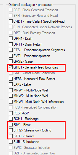
By aquaveo on June 19, 2019GMS allows using a number of different MODFLOW head boundary packages (GHB, RIV, STR, SFR, etc.) to indicate flow in or out of your model. These packages often appear to be similar. To the differences between them, here we discuss a few of these packages.
General Head
The General Head Boundary (GHB) is, conceptually, a fixed head far from the model where it is assumed to be a fixed head with time (i.e., the river or head will not be affected by the model stresses over time). The purpose of using this boundary condition is to avoid unnecessarily extending the model domain outward to meet the element influencing the head in the model. As a result, the general head condition is usually assigned along the outside edge of the model domain.
General head cells are often used to simulate lakes. General head conditions are specified by assigning a head and a conductance to a selected set of cells. If the water table elevation rises above the specified head, water flows out of the aquifer. If the water table elevation falls below the specified head, water flows into the aquifer. In both cases, the flow rate is proportional to the head difference, and the constant of proportionality is the conductance.
River
The MODFLOW River (RIV) package only tracks flow between the aquifer and the river. With the River Package, once water has entered the river, it is lost to the model.
Stream
Unlike the River package, the Stream (STR) package routes flow through the stream. The water can travel downstream and possibly re-enter the aquifer at another point. The Stream package also allow periodic drying. However, there are more restrictions than in the River package.
Also unlike the River package, the Stream package calculates the water depth based on the flow rather than it being manually entered. There are several different options available for calculating water depth, including using Manning’s equation or a depth versus flow table.
The Stream package divides streams into reaches and segments. It models effects of rivers on aquifers while tracking flow in river. Interaction between surficial streams and the groundwater for the Stream package uses Manning’s equation and simple channel hydraulics to compute the stage in the stream.
Streamflow Routing
This Streamflow Routing (SFR2) package is similar to the Stream package. Though it has more restrictions than STR, it has more sophisticated hydraulics and routing options.
These are just the most commonly-used of over a dozen different MODFLOW head boundary packages that can be used with GMS. Go ahead and explore the different MODFLOW packages available in GMS today!