Tips for Working with PEST
By aquaveo on April 17, 2019Parameter estimation using PEST can assist in data interpretation, model calibration, and predictive analysis. PEST can do a lot for your project.
Because PEST offers so much, it can be a little overwhelming to use at first. We provide tutorials and articles on our wiki to help guide you in using PEST with GMS.
In addition to the resources available in the tutorials and wiki, this post covers some useful tips that have helped some of our users.
General PEST Tips
Here are some general tips for troubleshooting PEST in GMS:
- Verify that the parameter key values have been successfully initialized under MODFLOW | Parameters. The key values should match the parameters names. For example, if the key value for hydraulic conductivity is “-30”, the parameter name should be “HK_30”. No key value should be used twice, even across different packages. To continue the example, if you have an “HK_30”, there should not be a “RCH_30”.
- Key values are needed for both zones and pilot points.
- Key values are expected to be negative integers. Non-integers will not be automatically recognized as key values.
- If the key value is not a negative integer, or is a parameter from the WEL package, they will have to be manually added. If you’re missing a value, check that it initialized in the first place.
- Parameters included in the run will be written to the *.param file. Once PEST runs, the optimal values are written to the *.par file.
- If the iterations are giving identical values for the same parameter, check if the value is either the minimum or the maximum of the range assigned to the parameter, then evaluate if that range needs adjusting.
- Adjusting the starting values or the PEST options may help.
Pilot Point Tips
When using PEST and pilot points, consider the following:
- Follow the recommended guidelines found here.
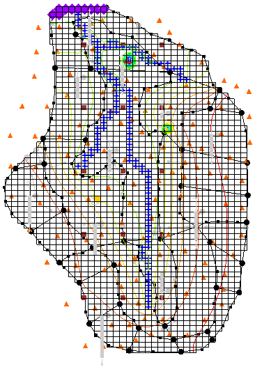
- You can get a quick 2D Scatter set to use for pilot points with the MODFLOW Layers → 2D Scatter Points tool. This is particularly useful for areal parameters, such as HK or RCH.
- If you’re running Null Space Monte Carlo, you must use pilot points and your interpolation method must be set to kriging.
- If running with SVD-Assist, you can point to the Jacobian file so it doesn’t re-solve for every iteration.
- Depending on the parameter, pilot points often should not start with zero values. This especially applies to log transforms.
We hope these tips help and that your project are improved by using PEST with GMS.