Aquaveo & Water Resources Engineering News

Troubleshooting Observations in GMS

After creating your observation points in GMS, have you ever reviewed the results from the observation wells and thought they didn't look right? It can sometimes happen that observation wells give back the wrong values or are missing altogether. This can happen for a number of reasons.

Here are a few tips to help ensure that your observation points give back accurate information:

Point Outside Grid
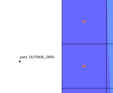
  1. Review the location of the observation points/wells. Make certain the point is located on the grid. A common issue is that the elevation of the point causes it to be above or below the grid, so be certain to review this.
  2. Make certain the observation points have correctly mapped over to the grid. If the point is outside of the grid area, then it will not be included in the model run.
  3. After being mapped over, check that the observation wells are in the correct layer of the grid. If the observation point is meant to be on more than one layer, make certain it shows up on each layer.
  4. Well Screen Equals Zero
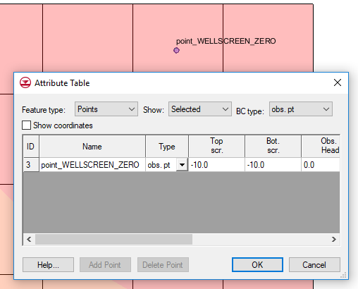
  5. When using a well screen, check the length of the point. If the length is 0, then the observation point will not be able to record any results. Check that the top screen elevation is higher (greater) than the bottom screen elevation by a positive, non-zero amount.
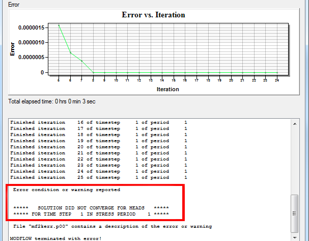
  6. Check that the observation point is in cells that are active. If there are no head values, or the cell is dry, then it is unlikely that the observation point will provide any useful information.

These are just some of the items to look for when using observation points in GMS. For most of these issues, when you save the file, a warning message should appear.

If you have a current license of GMS with paid maintenance, you may contact technical support for additional help in using observations. For project specific troubleshooting, contact Aquaveo's consulting team.

Blog tags: 

Using Advanced Data Services Options

In the current versions of GMS, SMS, and WMS, the data service options for importing online maps has changed. It was noted by some of our users that the Advanced option for the Data Services Options dialog was removed.

We are happy to say that the advanced options for the Data Services Options dialog has been restored. The new advanced options are only available when using the Import from Web command in the release of GMS, SMS, and WMS that went out at the beginning of May 2019.

To access the Advanced options from the Data Services Options dialog, click the Advanced button, just as before, to bring up the Select Online Source dialog. This dialog allows users to bring in new data sources for downloading data.

Select Online Source Dialog

Adding new data sources to the Select Online Source dialog can be done in any of three ways:

    Add New Source Dialog
  1. The Select Online Source dialog contains a list of all of the data sources currently available. You can select one of these sources and click the Duplicate Source button to create a copy of the data source. Then, with the copy selected, click the Edit Source button to reach a dialog where you can make modifications to the source such as limiting the layers downloaded from the source or changing the image format downloaded from the source.
  2. You can click the Add New Source button to reach a dialog where you can specify the url of a new data source along with any modifications.
  3. Finally, if you have an Online Source File with the information needed to reach a source, you can click the Add Sources from File to add the source to the available list.

Sources can be deleted from the available list by selecting a source in the list and clicking the Remove Source button. Only sources that have been manually added can be removed or edited.

To get access to the new advanced options for the Data Services Options dialog, visit our downloads page today.

Blog tags: 

What Makes a Good Quality Mesh?

Several models in SMS rely on using a 2D mesh. The quality of this mesh can greatly impact your model run and overall results, so here are some tips for making a good quality mesh.

Start with a Good Mesh Generator Coverage

A lot of how well a mesh turns out begins with the mesh generator coverage. Generally, when a poor mesh has been generated, it is because the arcs, vertices, and polygons on the mesh generator coverage did not clearly define a good quality mesh.

When defining the mesh parameters in the coverage, there are few items to keep in mind:

  • Make certain the polygons accurately reflect the work area. Do not draw polygons outside of your elevation data.
  • Vertices along the arcs determines the size and spacing of elements in the mesh. Adding too few or too many vertices along an arc can cause poor spacing. Using the Redistribute Vertices tool can help with getting the correct number of vertices, and making sure they are evenly spaced along each arc.
  • Keep individual arcs smooth and rounded to avoid interior acute angles.
  • Use the 2D Mesh Polygon Properties dialog to preview how the final mesh will appear.
Mesh generation coverage example
Check the Size Transition of the Elements

How elements transition in size can greatly impact how a model uses the mesh. In general, a gradual change in element size functions makes for a better mesh for most models. A poor mesh will have a quick change in elements size, acute interior angles, and thin triangles.

Mesh with incorrect spacing

The solution for smoothing out the element transition is to adjust the spacing of the arc vertices in the mesh generator coverage and to examine the proximity of the arcs. In general, arcs that are close to each other should have a similar number of vertices. Arcs that are further apart can have a greater disparity of vertices.

Mesh with corrected spacing
Check For an Even Patch

When creating quadrilateral elements in a mesh using a patch, it is important that the spacing of the vertices be precise. Parallel arcs need to have the same number of vertices when creating a patch or the result will be an uneven patch.

Example of an uneven patch

It is recommended to always preview the mesh when using the patch option, then adjust the number of vertices to make certain the patch is even.

Remove Unnecessary Elements

Cleaning up a mesh after it has been generated is sometimes necessary. When generating a mesh from a scatter set or other source, more of the mesh may need to be reviewed and cleaned. Using the Select Thin Triangles command and the Clean command can help with getting rid of unnecessary elements that could cause problems during the model run. It is also recommended to use a mesh with the fewest number of elements needed for your project.

These are only some of the recommended guidelines for generating a good quality mesh. We hope this helps you in your projects.

If you have questions about how to make a better mesh in SMS, contact our technical support for general questions, or contact our consulting services for project-specific inquiries.

Blog tags: 

Splitting UGrid Layers

Have you been working with a project in GMS only to discover that the project’s 3D unstructured grid (UGrid) needs to include another layer? Fortunately, it’s rare that a UGrid needs to have another layer, but every once in a while a layer needs to be added to an existing UGrid. GMS provides a way to divide UGrid layers quickly.

One thing to note: whenever a UGrid is changed—such as with adding a new layer—the existing MODFLOW simulation attached to the UGrid will be removed. It is therefore best to make certain the UGrid is correct—including having the necessary number of layers—before building the MODFLOW simulation.

In order to add a new layer to an existing Ugrid, do the following:

  1. Using the Select Cell tool, select a cell on the layer you want to split.
  2. Right-click on the selected cell and select the Split Layer command to start the process of dividing the UGrid layer.
UGrid layer before and after being split

When GMS finishes processing, it creates a new UGrid with the additional layer, leaving the original UGrid intact. The layer to which the selected cell belonged is divided into two layers on the new UGrid. GMS averages the distance between the top and bottom of the layer, then divides the layer equally to create the two new layers. It is recommended to carefully review the new UGrid to check for any unintended anomalies.

As mentioned above, any MODFLOW simulations contained in the original UGrid are not copied to the new UGrid. A new MODFLOW simulation must be created for the new UGrid.

Another option is to create a new UGrid with the additional layer and leave the existing UGrid as is. This option is best if you need to finely control the layer elevations.

For adding layers to complicated UGrids, you may want to consider using Aquaveo’s consulting services.

Now that you’ve seen the basics of splitting a UGrid layer, try it out in GMS today!

Blog tags: 

Modeling a Dam in GSSHA

Do you have a project that requires modeling a dam, or similar structure, in GSSHA? WMS can make this process smoother with tools designed to help define the structure quickly and efficiently.

In order to create a simulation that includes modeling the dam in WMS and analyzing the dam’s effects using GSSHA, the workflow is as follows:

  1. Import an existing GSSHA base model.
  2. In the GSSHA map coverage, use the Shift key to select the node where you want the dam to be and the node immediately downstream from it.
  3. Right-click on the selected nodes and select Attributes to open a Properties dialog.
  4. Select Output Hydrographs at those nodes.
  5. Run GSSHA.
  6. Using the results from the GSSHA run, size your embankment based on the necessary storage.
  7. Using the Create Feature Arc tool, create an arc to represent your dam.
  8. Double-click on the arc to bring up the Attributes dialog.
  9. Set the type of arc to be an Embankment, then click the ... button next to it to open the Embankment Arc Profile Editor dialog.
    1. Set the PVI Elevation to be the height of the dam.
    2. Click Compute Vertical Curve to compute the Curve Length.
  10. Double-click the node in the stream where your structures will be defined to open the Properties dialog.
  11. Click the button under Hydraulic structures to open the GSSHA Hydraulic Structures dialog.
    1. Add a Detention Basin, Weir and Culvert.
    2. Define the attributes for each of these structures.
  12. Run GSSHA again to see the effects of the dam you have created.
GSSHA Dam Modeled in WMS

If needed, adjust the display options when reviewing the results to get a better idea of how the dam structure affected the results. Try different various options to get a better feel of how the dam affected the simulation results.

Now that you know how to add a dam to GSSHA, try out modeling dam structures and other applications in WMS today!
Blog tags: 

Using the Snap Preview Option

Having trouble with your boundary conditions or materials not aligning correctly with your mesh?

When a simulation runs in SMS, it takes all of the components—such as boundary conditions and materials—and aligns them with the 2D mesh or other geometry. When creating boundary conditions in the Map module for SRH-2D, ADCIRC, or other models that use simulation components, it can sometimes be difficult to know exactly where the boundary conditions will line up with the 2D mesh nodes.

To help with this, the boundary conditions map coverage contains a display option to see how the map arcs and mesh nodes will line up: the Snap Preview option.

To use the Snap Preview option, do the following:

  1. Make certain the project contains a 2D mesh and a boundary conditions coverage that have been linked to a model simulation
  2. Open the Display Options dialog
  3. On the Map tab of the dialog, turn on the Snap Preview option

The Snap Preview option can also be turned on or off by using the Shift+Q shortcut key.

When the Snap Preview option has been turned on, a dashed line will be displayed along the element edge to show where the boundary condition arcs will match up with the mesh nodes. This is helpful in identifying if the placement of the boundary condition arcs is correct. Incorrect placement of boundary condition arcs can cause errors in the model run.

Snap Preview Example

The Snap Preview option also works for other model coverages such as the SRH-2D materials coverage. This allows previewing how material assignments will match up with the mesh elements. Adjustments can then be made to the material polygons to correct any misalignments.

Using the Snap Preview option can significantly reduce frustration and prevent errors early on. Try using Snap Preview in your SMS projects today!

Blog tags: 

Tips for Working with PEST

Parameter estimation using PEST can assist in data interpretation, model calibration, and predictive analysis. PEST can do a lot for your project.

Because PEST offers so much, it can be a little overwhelming to use at first. We provide tutorials and articles on our wiki to help guide you in using PEST with GMS.

In addition to the resources available in the tutorials and wiki, this post covers some useful tips that have helped some of our users.

General PEST Tips
Model calibrated using PEST

Here are some general tips for troubleshooting PEST in GMS:

  • Verify that the parameter key values have been successfully initialized under MODFLOW | Parameters. The key values should match the parameters names. For example, if the key value for hydraulic conductivity is “-30”, the parameter name should be “HK_30”. No key value should be used twice, even across different packages. To continue the example, if you have an “HK_30”, there should not be a “RCH_30”.
  • Key values are needed for both zones and pilot points.
  • Key values are expected to be negative integers. Non-integers will not be automatically recognized as key values.
  • If the key value is not a negative integer, or is a parameter from the WEL package, they will have to be manually added. If you’re missing a value, check that it initialized in the first place.
  • Parameters included in the run will be written to the *.param file. Once PEST runs, the optimal values are written to the *.par file.
  • If the iterations are giving identical values for the same parameter, check if the value is either the minimum or the maximum of the range assigned to the parameter, then evaluate if that range needs adjusting.
  • Adjusting the starting values or the PEST options may help.
Pilot Point Tips
PEST with pilot points

When using PEST and pilot points, consider the following:

  • Follow the recommended guidelines found here.
  • You can get a quick 2D Scatter set to use for pilot points with the MODFLOW Layers → 2D Scatter Points tool. This is particularly useful for areal parameters, such as HK or RCH.
  • If you’re running Null Space Monte Carlo, you must use pilot points and your interpolation method must be set to kriging.
  • If running with SVD-Assist, you can point to the Jacobian file so it doesn’t re-solve for every iteration.
  • Depending on the parameter, pilot points often should not start with zero values. This especially applies to log transforms.

We hope these tips help and that your project are improved by using PEST with GMS.

Blog tags: 

Modeling a Dam in WMS for Use in HEC-HMS

Do you have a project that requires modeling a dam, or similar structure, in HEC-HMS? WMS can make this process smoother with tools designed to help define the structure quickly and efficiently.

This blog presents a workflow for modeling a dam in WMS to later analyze in HEC-HMS. The workflow is as follows:

  1. Begin with a delineated watershed with attributes defined.
  2. Determine where you would like to place your reservoir and place an outlet point there.
  3. Delineate your watershed and compute basin attributes using your new outlet point.
  4. Create a simulation in HEC-HMS and compare the runoff from the upper basin to the lower basin in order to size your reservoir.
  5. Convert the outlet node to a reservoir.
    1. Switch to Hydrologic Modeling Module.
    2. Using Select outlet tool, select the outlet at the location where you want to model a reservoir.
    3. Right-click and select Add | Reservoir.
  6. Select Calculators | Detention Basins.
  7. Click Define to bring up Storage Capacity Input.
    1. For a dam: Use DEM and enter the height of the desired dam.
    2. Click OK to exit Storage Capacity Input dialog. The Detention Basin Analysis dialog will appear.
    3. Define the storage curve for your reservoir.
    4. Click Map to Hydrologic Model to open Map to Model. Name the series as desired.
  8. Double-click on the reservoir point to open the HMS Properties dialog.
    1. Here, you can choose the storage curve defined earlier, and define all other curves.
    2. To add an orifice to your dam, select Orifice Outlet from the Outlet Type drop-down.
      1. Define the orifice Center Elevation, Cross-sectional Area, and Discharge Coefficient.
    3. To add a spillway, select Broadcrested Spillway or Ogee Spillway from the Spillway Type drop-down.
      1. Define the required characteristics for the selected spillway.
    4. You can also choose to model an overflow type and dam break type if desired.

With the dam, spillway and orifice defined, you can now run your model through HEC-HMS again to see how your reservoir will perform under the selected storm.

Dam analysis in HEC-HMS

Try out modeling dam structures and other applications in WMS today!

Blog tags: 

Using the Simulation Run Queue

SMS allows having multiple simulations for the same project with models such as SRH-2D, ADCIRC, and STWAVE. Furthermore, SMS 13.0 lets you run and manage multiple simulations running at the same time using the new Simulation Run Queue dialog.

Simulation Run Queue

The Simulation Run Queue is a modeless dialog, meaning you can continue using SMS while simulations are running. Once a model run has started for a simulation, you are free to start building a new simulation, even one using the existing components. Completed runs may be visualized in SMS while additional runs are still in process.

Functionality

The new Simulation Run Queue dialog functions a little differently from the previous Model Wrapper dialog. Some of the changes include:

  • You must click Load Solution to load the desired simulation solution into the project. This does not happen automatically when you click Close as it did before.
  • If you try to run a simulation already in the queue, you will be prompted to remove the simulation from the run queue before it can be run again.
  • If changing an active simulation’s settings, renaming the active simulation, or taking any action that affects a simulation currently in the queue, you will be asked to remove the simulation from the queue prior to making the changes.
Viewing Plots

With the Simulation Run Queue, diagnostic information—such as monitoring plots—can be displayed during model runs. By turn Monitoring Data off or on, you can watch command line results and residual plots.

Options also exist for changing which plots are displayed in the run queue. Selecting a simulation causes the Plot Options button to appear. In the Plot Options dialog, you can choose which plots to view. You can view Residuals, Monitor Points, and Monitor Lines, and change the options associated with each of these.

Now that you know a little more about the Simulation Run Queue dialog in SMS 13.0, try it out today!

Blog tags: 

Troubleshooting MODFLOW, Part 2

A while back on this blog, we discussed troubleshooting MODFLOW errors. That blog post specifically discussed making use of the Model Checker, the MODFLOW command line output, and the output file. It also gave a few tips on how to fix your model when an error is encountered.

We wanted to expand on this, and specifically discuss what to do when you model doesn’t converge. When the model does not converge, an error message should appear in the MODFLOW command line output.

MODFLOW Not Converging

Essentially, when a model doesn’t converge a component of the model has not been setup correctly. This inaccurate component may only cause the model to not converge when certain conditions have been met, but otherwise the model will converge when those conditions are not present.

As for why your model converges sometimes and not others, there are a wide range of possible causes for instability. Here are a few general suggestions for helping MODFLOW converge:

  • Check model inputs for reasonableness.
  • Try running the model with different solvers. There are several solvers to choose from, and each of them have their own strengths and weaknesses. To switch solvers, select MODFLOW | Global Options | Packages and then select a different solver in the lower left area of the MODFLOW Packages dialog.
  • Try changing the solver parameters.
  • Check the troubleshooting items for a model that is not converging can be found under item K of the Frequently Asked Questions section of the Online Guide to MODFLOW.
  • Deselecting the "Enable saving of computed flows for all source/sink objects" option in the MODFLOW Output Control dialog.
  • Reduce the time step length for the model run.

It can take some time to review the model to discover why it is not converging, but the effort it worth it for an accurate result. For more in-depth assistance with model troubleshooting, please consider reaching out to Aquaveo’s consulting team.

Blog tags: 

Pages