Aquaveo & Water Resources Engineering News

Reducing Scour in SRH-2D Sediment Transport

Do you have an SRH-2D sediment transport model that has an unreasonable amount of scouring? There could be several different issues in your model that are causing unreasonable scouring, however, SMS contains several different ways to fix this issue. This article will cover how to limit scouring so it is put to extremes in your model.

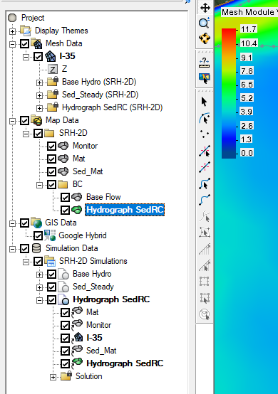
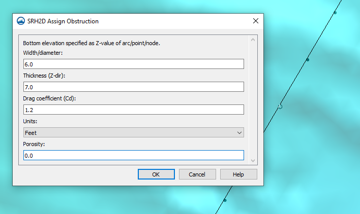
  1. Review the sediment loading on your boundary conditions for the sediment transport model. Double-click on one of your boundaries to check your sediment boundary conditions to review how the sediment loading has been defined. In the SRH-2D Assign BC dialog check and update the Sediment inflow section if needed.
  2. Example of scouring within an SRH-2D sediment transport model. The image on top shows the scour and the lower image it has been fixed.
  3. For your sediment transport SRH-2D simulation, go to SRH-2D Model Control and select the Sediment tab. Review the Particle diameter threshold section to make certain that the sizes are reasonable. Often having diameters that are too large causes scouring.

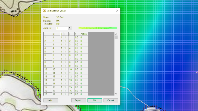
  4. Another place to review is the SRh-2D sediment material coverage. Right-click on the click Materials List and Properties. Under Gradation Curve, right-click on one of the materials and select click Edit Curve to bring up the Gradation Curve dialog. Review the gradation values and check for inconsistencies. Remember that the values need to be scaled from the smallest sand to the largest boulder. It is important to remember that the maximum number of functioning rows only goes up to nine. Any more than this will cause inconsistencies to appear.

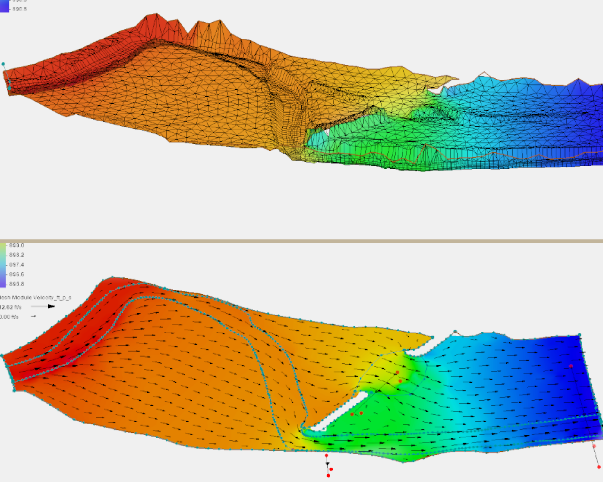
    When the values that are entered in the Sediment Gradation Parameters are put to extreme values this is what will often cause the deep scour you may see in your model. A regular model will be smooth with very little deviation. A helpful resource to use if things are still not clear is the USBR website. They have example problems that you can follow.

These are just some of the tips for reducing scouring in your SRH-2D sediment transport models. For additional support for sediment transport with SRH-2D contact our technical support team. Try out SRH-2D with sediment transport in SMS 13.2 today!

Blog tags: 

Exporting Using the View Values Command

In your groundwater model in GMS, do you need to export only a specific dataset value? GMS provides a way for you to export different dataset values and save them as text files that you can continue to edit outside of GMS. This post will cover exporting values using the View Values command.

To export data using the View Values command, select a dataset in the Project Explorer then right-click and select the View Values command. This will open the Edit Dataset Values dialog. This dialog shows an array of data values for the selected dataset. From the Edit Dataset Values dialog, you can export the data values in a couple ways.

Example of the Edit Dataset Values dialog

The first option is to click the Export button in the dialog. This will open the Dataset Filename dialog. Here you can give the exported file a name and save out the data as a tabular text formatted file. This exported file can be opened with a text editor or spreadsheet program. All values in the dataset will be exported with this value.

The second option is to select the data in the data array, then copy (Ctrl+C) and paste (Ctrl+V) the values into another document such as Excel or Google Docs. This method gives you the option to be selective about which data values to include. This method also allows you to save out the data in other file formats.

It is important to note that if you change the formatting in the text file, in excel, or google sheets and try to import the file back into GMS it may not import correctly. The format used in the Edit Dataset Values dialog is the format that GMS will be expecting when importing the data back into the project.

Try out exporting dataset values using the View Values command in GMS today!

Blog tags: 

Tips for Watershed Delineation

Having a well delineated watershed basin can make a difference in your watershed model. WMS contains a method to automatically delineate a watershed for your projects. This tool can quickly create a delineated basin so you can move on with your watershed projects. This post will cover the different tips on how to help you successfully delineate a watershed basin in WMS.

Try switching between TOPAZ and TauDEM
Example of the Watershed Delineation Wizard in WMS

If using either TOPAZ or TauDEM fails to give you a valid watershed basin, try using the other. Switching between TOPAZ and TauDEM can help with delineating your watershed, however, it does depend on what you need for preprocessing. It is important to remember that TauDem can only work for pulling out streams, it does not work for ridges. This is why in most cases it is better to use TOPAZ. These tools both can take a while to run so it is best to get this process done as soon as possible.

Check the resolution of your DEM

If the resolution is too low on your DEM then it is unlikely that it will properly generate the data files. You can fix this by choosing a DEM that has a higher resolution. However, it is important to note that if the resolution is too high it may take too long for the data files to load and for the delineation process to finish. It is best to find a happy medium between the two so the data files will load, the delineation will go quickly, and the resolution will still hold up.

Adjust your outlet location

In order to delineate a watershed, you will need a place for all the water to end up flowing to. A misplaced outlet point can cause issues with the delineation process. Adjusting the location of the outlet point can improve the final basin results.

Try out delineating watershed basins on your project in WMS 11.1 today!

Blog tags: 

Tips for Organizing the Project Explorer in SMS

SMS has many kinds of datasets, geometries, and simulations that could be added to your Project Explorer. These are useful features with essential roles in building a valuable project in SMS. But sometimes the Project Explorer gets very full and becomes difficult to navigate. This is when it can be useful to organize the Project Explorer to make things easier for you and those you work with. Today, we have some tips on how you might keep things organized so you can accomplish what you need to.

Example of Project Explorer Organization in SMS
  1. You might find it useful to name each new project element with a name that helps describe it. Descriptive names can help you find your project elements more quickly when you need to tweak something here or there. For example, you might have a materials coverage where the default Manning’s n is 0.015 and another one where you’ve changed it to 0.045. Labeling the materials coverage “n-0.015” and “n-0.045” could help you remember the difference between the coverages.
  2. You can add folders to organize items in the Project Explorer. For instance, you could group coverages according to which simulation you intend on using them for. Or maybe you have already imported a couple of rasters that you only need for one element of your project. You could put them together in a folder and collapse the folder in the Project Explorer. This will keep them out of sight while you don’t need them and could help you find them faster once you do need them. Note that solution data is automatically organized in folders in coordination with each simulation in the project.
  3. You can add notes to most elements of your project. To add a note, use the Properties… right-click command on an item in the Project Explorer and go to the Notes tab. There, you can leave notes for your colleagues (or yourself) about the item’s intended use or provide additional information that is not readily apparent. This is particularly helpful with simulations when you can add a note giving a summary of the key features of that simulation. Notes could also be used to indicate datasets you compared to get a new dataset. These can help everyone keep track of what function each thing serves in a given project.
  4. As you go through the project, it is recommended to delete what you’re not using. Not only does this organize the Project Explorer, it also frees up space in SMS. This can help you avoid slow processing time that can come from too many simulations. In general, we recommend you not have more than seven simulations in a project. It is also recommended to remove large rasters, shapefiles, or images after you are done using them. If you want to keep certain elements that you’re not using right now, you may want to minimize them or put them in a folder when not in use.

Using these tips, you will keep your projects organized and accessible. Make use of the organization tools for the Project Explorer in SMS today!.

Blog tags: 

Using Exchanges with MODFLOW 6

How can you get models to run smoothly together in MODFLOW 6 in situations where boundary conditions don’t adequately describe their relationship to each other? In MODFLOW 6, you have the option of relating models to each other through an exchange instead of just using boundary conditions. This allows the MODFLOW 6 to calculate the flow between each model as if it were part of one large unstructured grid.

Connecting models through exchanges allows for the transfer of information back and forth between two models with distinct purposes and packages. GWF-GWF Exchanges create relationships between the cells of GWF Models by identifying cells where water will be exchanged between. The GWF-GWT exchange creates a relationship where the GWF Model provides the flow data that informs the GWT Model.

Example of the GWF-GWF Exchange Options

But in what situations might you use these exchanges?

In the case of GWF-GWF Exchange, the USGS has identified several situations where this could be desirable:

  • Horizontally adjacent models: It may be necessary to connect models that are in the same area in order to better describe how they relate to each other.
  • Vertically adjacent models: As with the horizontally adjacent models, it may be better to connect models that represent different layers more completely than it is to simply put all the layers on one model. This allows for variation in the fineness of the grids while maintaining communication between them all.
  • Locally refined grids: You might want to refine grids around areas where you want more specific results. Using an exchange, the simulation will calculate them all like they’re part of the same unstructured grid.
  • Periodic boundary conditions: This use aims to show the effects of repeating conditions by coupling cells on opposite sides of the model. Instead of exchanging information between cells of adjacent or circumscribing models, you can exchange information between cells in the same model that are not already adjacent to each other.

As mentioned above, the primary purpose of the GWF-GWT exchange is to provide the flow information from the GWF Model to the GWT Model. Since the GWT Model needs flow data for every cell in the model, this is a convenient way to provide that flow data. (For extended information on inputting data for GWT Models, see USGS documentation).

If you have MODFLOW 6 models that you would like to connect to each other, experiment with exchanges in GMS 10.6 today!

Blog tags: 

Introducing the Toolbox in SMS 13.2

One of the new features added to SMS 13.2 is the Toolbox. The addition of the Toolbox allows multiple tools to be collected into one location. Many of these tools previously existed in other locations in SMS such as the Dataset Toolbox. In addition to these tools new tools have been developed for the Toolbox.

You can access the Toolbox using the Toolbox macro button located on the macro toolbar. Clicking the macro will open the Toolbox dialog containing a list of available tools.

The tools have been organized into folders in the Tools tab. Examples of folders include: Coverages, Datasets, Rasters, and Unstructured Grids.

  • Coverage tools are used to manipulate coverages and feature objects.
  • Datasets tools are many of the tools that have previously existed in the Dataset Toolbox and are used to manipulate datasets.
  • Rasters and Lidar tools are used to adjust and clean up raster and lidar data.
  • Unstructured Grid tools can manipulate and adjust unstructured grids (UGrids).
Example Compare Dataset Tool in the Toolbox for SMS 13.2

In addition, there will be folders for manipulating data related to specific numeric models. For example, there is a folder with tools that work with ADCIRC data.

The Toolbox also contains a History tab. This tab keeps a record of all the tool runs used with your projects. As a result, it allows you to run the same tool again using the same settings. For example, you might use the Compare Dataset tool to compare the solution sets from two different simulations, then discover that there was an issue in one of the simulations. After you fixed the simulation and ran it again, you could use the history feature of the toolbox to run the Compare Dataset tool using the same settings as before.

The History tab also shows if a tool executed successfully or not. Furthermore, it lets you make notes on the different tool runs, allowing you to clarify why a tool run failed or what you were hoping to accomplish with a particular tool. This can facilitate collaborating with colleagues when working on the same project.

Additional tools will be added to the Toolbox in future versions of SMS. Try out the Toolbox in SMS 13.2 beta today!

Blog tags: 

Announcing SMS 13.2 Beta

We are pleased to announce that SMS 13.2 has been released in beta. SMS 13.2 beta includes many new features to aid in your surface-water projects. Here are a few of the new features we’re excited about.

SRH-2D Improvements

SMS continues to add support for SRH-2D. SMS 13.2 has improved support for modeling HY-8 structures as links to allow for 2D flow overground.The sediment transport options have also been improved. Additional tools for SRH-2D include calibration options and report generation.

New Toolbox

A new toolbox has been added giving you more options for adjusting and manipulating data in your projects. The toolbox contains many of the tools that are in the Dataset Toolbox with the addition of several more tools. Additional tools will be added to this toolbox in future versions of SMS.

Example of the Toolbox in SMS 13.2
Display Themes

The Display themes tool allows you to save your display options settings which can be reused later or applied to other models. Specific display options and views can be saved as display themes. Furthermore, you can have multiple display themes in a project. This makes it easier to switch between different regularly used displays.

UGrid Clipping

SMS continues to improve its features for unstructured grids (UGrid). The UGrid module now has an additional option for clipping. This option can be found in the UGrid Display Options. Turning on the UGrid clipping option allows you to create a "clipping widget" that you can use to hide part of your Ugrid. Primarily this feature allows you to view cross sections of a UGrid.

Model Interface Updates

The interface for a couple models have been updated. This includes CMS-Wave and TUFLOW-FV. These interface updates make use of workflows similar to CMS-Flow and SRH-2D. Additional functionality has also been added to these models.

These are just a few of the features that are a part of SMS 13.2 beta. Try out these features and many more by downloading the SMS 13.2 Beta today!

Blog tags: 

Having Multiple MODFLOW 6 Simulations in GMS

Have you tried including multiple MODFLOW 6 simulations in your GMS project? Having multiple MODFLOW 6 simulations allows you to run simulations for the same area. This can help with calibration, making comparisons, and troubleshooting a model. This post will cover how to keep things organized when using multiple simulations in a single project file.

After you have created a second MODFLOW 6 simulation, it is recommended that you give the simulation a name that will help you remember the purpose of that simulation. For example if you have a base simulation that you are using to create a stable starting run, it could be named something like “Base_Sim”. If you then create a second simulation that has a longer run time, naming it something like “Base_Longer_Run” might be helpful.

Furthermore, you can use the Notes feature available in the simulation properties dialog to add notes about what makes each of the simulation unique. This can be particularly helpful when sharing the project with coworkers.

In some cases you may have multiple UGrids. For example, you may want to use one UGrid that is less refined for a simulation for a base simulation and a more refined UGrid to test with a duplicate simulation. When doing this, be certain to correctly name the UGrids so that they are easy to tell apart. Also, make certain the UGrid is linked to the correct MODFLOW 6 simulation. It is usually best to create a separate simulation for each UGrid.

Often when using multiple simulations, you will want to have specific map coverages applied to specific simulations. When doing this, you can organize your coverages in the Map module using folders. Using folders can help keep straight which coverages belong with which simulation. And can also help in keeping the Project Explorer from becoming cluttered.

Example of Multiple MODFLOW 6 Simulations in GMS

In the Project Explorer, collapse any folder that you are not currently using. This will help keep the Project Explorer free of any unnecessary clutter. This is particularly helpful when you have solution data from different simulation runs. GMS will automatically place simulation solution files in their own folder in the Project Explorer under the UGrid connected to that simulation, as well as as links under the simulation. Additional folders can be added to organize solution data.

Also, when working with multiple simulations, it can be helpful to lock simulations that are not currently being worked on to reduce chances of accidentally making changes to the wrong simulation.

It should also be noted that having too many simulations in a project can cause GMS to run slowly. It is typically recommended to have fewer than seven simulations in a project.

Having multiple MODFLOW 6 simulations in your project expands your groundwater modeling options. Try out using multiple MODFLOW 6 simulations on your project in GMS today!

Blog tags: 

Tips for Building a CE-QAUL-W2 Model

Are you building a CE-QUAL-W2 model in WMS? CE-QUAL-W2 is a 2D laterally averaged hydrodynamic and water quality model. It can model vertical variance, eutrophication, seasonal turnover, algal blooms, etc. if incoming pollutants are known. Setting up a CE-QUAL-W2 simulation involves dividing the reservoir into segments, branches, and layers and determining the geometric properties of each segment, branch, and layer.

When building a CE-QUAL-W2 model, keep the following in mind:

  • Make certain that the site you have chosen is appropriate for the CE-QUAL-W2 numeric model. It is best applied to long and narrow water bodies that have longitudinal and vertical water quality gradients. The further your site location deviates from a long and narrow water body, the less ideal it is to CE-QUAL-W2.
  • Example of smoothing an arc for a CE-QUAL-W2 model
  • When setting up branches, you may need to remove smaller branches and offshoots. This may particularly be the case if you used the TIN Boundaries to Features command. Using this command can end up including small branches and offshoots that are unnecessary for the final model. Each branch should be examined and judgment exercised on the importance of including it in the model. To remove the unnecessary branches, smooth out the bounding polygon.
  • Before smoothing out a bounding polygon, it is recommended that you duplicate the original map coverage in order to retain the original coverage data. Then use the map tools to smooth out the bounding polygon for the coverage that will be included in the model. Remove any extra coverages when you finish smoothing the bounding polygon.
  • Verify that all segments are measured and assigned correctly. This is done by double-clicking on any segment in the segment coverage and using the Polygon Segment Attributes dialog to review each of the segments. Either enter values for segments that are missing attributes or remove the segment.
  • Review branches through the Polygon Branch Attributes dialog. This is accessed by double-clicking on any branch in the branch coverage. Make certain to enter values for all branches.

Using the tips above can help assure that your CE-QUAL-W2 model executes correctly. For additional support, contact our technical support staff. Try out CE-QUAL_W2 in WMS today!

Blog tags: 

Understanding SRH-2D Obstructions

Do you have an SRH-2D project that might benefit from using obstruction objects? The obstruction coverage in SMS allows you to add obstruction objects to your SRH-2D project. Using obstructions in some cases can be beneficial, but there are a few key ideas to keep in mind. This post will cover some of these.

Adding obstructions to an SRH-2D project involves creating a coverage assigned as an SRH-2D obstruction type coverage. On this coverage, you can draw arcs and points to act as obstruction objects. Each arc and point can be assigned obstruction attributes. Finally, the obstructional coverage can be added to the SRH-2D simulation to be used in the model run.

Example of the SRH-2D Assign Obstructions dialog

First, it is important to understand how obstructions interact with the model run. Obstruction objects on the obstruction coverage will reduce the flow of water through the model by applying a drag force. Water will not flow around the obstruction but will instead be slowed by the drag force of the obstruction. The assigned attributes on the obstruction object will determine which cell nodes on the mesh will be assigned as an obstruction. Obstructions can be used for items like bank protrusions and boulder clusters.

Second, when assigning obstruction attributes to an obstruction object, a width/diameter is specified in SMS. For point obstructions, this user-specified value is then converted by PreSRH-2D to a radius for SRH-2D. The SRH-2D model applies the radius around the point. For line obstructions, the arc definition and width are converted by PreSRH-2D to point locations that define the obstruction area. That means, for example, if you assign an arc to have an obstruction width/diameter value of 2 meters, then 1 meter on one side of the arc and 1 meter on the other side of the arc will be the obstruction area.

Third, obstruction objects can be assigned a drag coefficient, porosity, and a specific thickness. It is important to note that obstruction objects are not meant to completely impede the flow of water.

For items that completely block the flow of water, such as bridge piers or buildings, a void in the mesh should be created that models the area of blockage in most cases. Likewise, having a large number of obstruction objects in your model sometimes can cause issues with the SRH-2D model run and therefore it is recommended that obstruction objects be used judiciously.

Obstructions can be a valuable addition to your SRH-2D model. Try using obstructions with SRH-2D in SMS today!.

Blog tags: 

Pages