Using CAD Data to Delineate a Watershed
By aquaveo on April 11, 2023Did you know that you can use CAD files to delineate your watershed area in a Watershed Modeling System (WMS) project? WMS is capable of using CAD data for elevation data, designs, layouts, and more. CAD data can be converted to TINs and feature objects to be implemented in a WMS project.
When converting the CAD data to feature objects, you can choose which layers from the data you would like to use when creating the new feature object. After that, you can clean up the feature object and choose all the properties for the coverage. To convert CAD data into feature objects, do the following:
- Import the CAD data into WMS from a DWG, DXF, or DGN file.
- After importing the CAD data, review the data to verify that it was imported correctly and that it has the correct projection.
- Right-click on the file in the Project Explorer and select Convert | Feature Objects….
- In the Cad → Feature Objects dialog, select which layers to convert into feature objects.
- Make certain the new coverage is set to have the "drainage" type.
- Designate the converted feature objects as outlet points and streams. Also verify that any stream arcs a set with the correct direction.
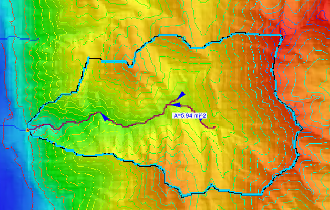
With the CAD data converted to feature objects and you've designated your outlets and streams, you can start the process of delineating your watershed. To do this, you will need a DEM in your project. If you have elevation data stored in a CAD file, you will first need to convert the CAD data to a TIN.
CAD data can be converted into TIN points or TIN triangles, but the best way to end up with TIN triangles is to convert into TIN points first. To convert CAD data directly into TINs, do the following:
- Import the CAD data into WMS in the form of a DWG, DXF, or DGN file.
- Right-click on the file in the Project Explorer and select Convert | CAD Points → TIN Points.
- In the Cad → TIN dialog, select which layers to convert and the name the TIN data will appear under in the Project Explorer.
- Right-click on the TIN point data in the Project Explorer and select Triangles | Triangulate.
From here you can convert the TIN to DEM if necessary. The TIN module in WMS has a few tools for working with basins that may be sufficient for your model. However, some models either perform better or require a DEM. Once you have the DEM you can generate the delineated basin. To do this:
- Right-click on the TIN and select Convert | TIN → DEM.
- Enter parameters for the DEM in the Convert TIN to DEM dialog.
- Review the generated DEM.
Once you have a DEM, complete the following steps:
- Select DEM | Compute Flow Direction in the Drainage module.
- Select DEM | Polygon Basin IDs →> DEM in the Drainage module.
- Select DEM | Compute Basin Data in the Drainage module.
Once you have a delineated basin, you can use the basin with the watershed modeling model of your choice. Be certain to review the basin to make certain it contains all of the area you need for your project.
Head over to WMS and see how you can utilize CAD data to create delineated basins in your projects today!
>