Using the SMS Toolbox History Tab
By aquaveo on November 2, 2022The SMS toolbox has a lot of tools to suit your modeling needs, from adjusting ADCIRC levees to calculating a Manning's n dataset. In some cases you might need to run one of these tools repeatedly with only slight modifications to the settings. The History tab of SMS's toolbox can make that process a lot simpler. This article discusses how the History tab of the Toolbox dialog facilitates your use of the SMS toolbox.
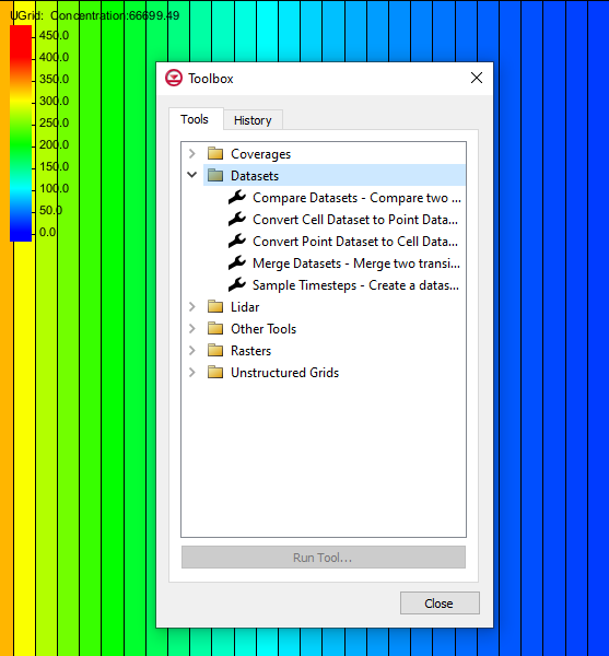
The History tab of the Toolbox dialog saves each run in the current project of each tool from the SMS toolbox. From the History tab, you can open any tools that have been run in the currently open project with the settings from that run. To do so, select the Toolbox macro, then the History tab of the Toolbox dialog. The tool runs are categorized under folders labeled with the date on which they were run. The History tab also displays the input and output for each tool. That information can be accessed by clicking the arrow to the left of the tool. To open the tool with the settings from a given run, select that run from the History tab.
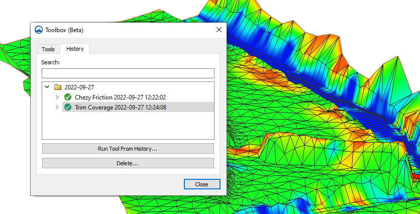
There are lots of situations in which the History tab might be useful. For example, it's possible that you need to trim several coverages with the same trimming coverage, the same buffer distance, and the same trimming option. Once you've run the Trim Coverage tool the first time, you can navigate to the History tab of the Toolbox dialog and select the run of the tool that you just completed. Once in the Trim Coverage dialog again, all you have to do is edit any settings that need to be changed for this specific run. From there, you can run the tool because all the other settings needed were saved from the last run.
But what if you've run many tools in this project, and you can't find the tool run you're looking for? Wouldn't it be easier to just specify the settings in the tool again? Possibly, but you don't have to dig through each run of every tool trying to figure out which run was which. The History tab of the Toolbox dialog has a search function that can search the input and output parameters for every tool in the History tab. It narrows down the tool runs to the ones that have information matching your search. So if you remember the name of an input coverage (or any other option), you can get a lot closer to finding the tool run you are looking for.
Note that the History tab of the Toolbox dialog saves information in the project you are currently working on. This means that the project always has a history of the tools that have been run in it. However, it also means that the tool history information doesn't transfer between two projects.
In sum, the SMS toolbox gives you tools for automating certain tasks in your SMS project; the History tab of the Toolbox dialog helps you save time while using these tools. Try out the SMS toolbox in SMS 13.2 today!