Defining Hydraulic Conductivity for Specific Layers
By aquaveo on January 26, 2022In your groundwater model, do you need to define hydraulic conductivity for specific layers differently than other layers? Do you need to modify the hydraulic conductivity values for specific areas within a single layer? GMS provides more than one way to assign hydraulic conductivity. This capability gives you more precision with regard to how hydraulic conductivity is assigned to your groundwater model.
Using the conceptual model approach, hydraulic conductivity can be assigned to polygons on a single coverage then mapped to your model. You can also use multiple coverages, assigning the hydraulic conductivity to specific layers ranges. The workflow for this is as follows:
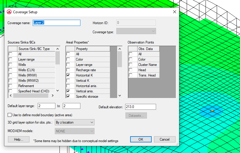
- Right-click on the coverage and select "Coverage Setup...".
- In the "Default Layer range" set the layer range you would like to use.
- Select the coverage to make it active.
- Double-click on a polygon within the coverage.
- It will bring up the attribute table for that group of layers.
- Set the conductivity for the polygon.
- Repeat this process for each desired group of layers.
When using this workflow, take care to make certain you are setting the correct attributes to the correct layer of your grid. Naming the coverage with the layer number or layer range can help with this process. You may also want to use the notes feature to attach reminders as to how the coverage has been set up.
It should be noted that when mapping multiple coverages to your grid, GMS follows an order of priority for the coverages. If you have different conductivity values on different coverages that overlap it is recommended that you apply the coverages individually. The last coverage that you apply will overwrite any overlapping values. If you apply all the coverages at once, the conductivity values will be summed up in areas where they overlap.
Try out using multiple coverages to define hydraulic conductivity for specific layers in GMS today!