New Project Explorer Commands for SMS 13.1
By aquaveo on April 14, 2021With the release of SMS 13.1, you might have noticed a few new commands in the Project Explorer right-click menus. The Project Explorer, or data tree, in SMS contains a list of modules and objects that have either been imported into the project or created in the project. Right-clicking on any of these objects will produce a number of commands to perform specific functions or launch certain tools.
Over the development of SMS, the number and type of commands in the Project Explorer have fluctuated. Changes are made to enhance the use of SMS. With SMS 13.1, new commands can be found when clicking on the Project icon at the top of the Project Explorer.
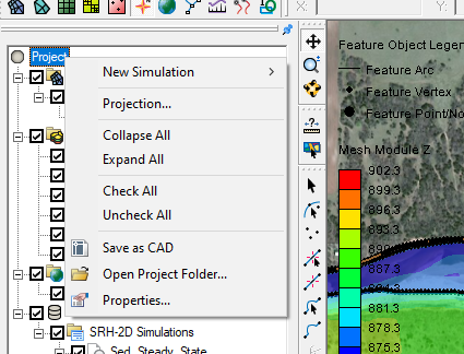
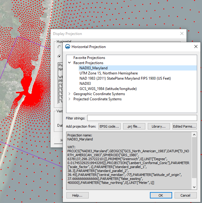
In this new right-click menu, you will find several commands that have become common in other Project Explorer right-click menus. These include a New Simulation sub-menu and a Projections command. The Projections command will open the Display Projections dialog to set the projections for the entire project. There is also an Open Project Folder command that will open a file explorer window to show the location of the saved project. A Properties command has been added to see details about the project, and contains a place to make notes about the overall project.
These commands also include collapsing or expanding all of the objects in the project. For the Project menu, this would collapse all of the items so only the Project icon is shown, or expand the data tree to show all objects in the project. There are also commands to toggle off or on all data in the project.
Finally, there is a new command, the Save as CAD command. This command will allow you to save a CAD file that contains CAD data generated from all visible data in the Graphics Window.
The new right-click menu commands give you more options for working with data in the Project Explorer. Try this out in SMS 13.1 today!