Aquaveo & Water Resources Engineering News

Using Interpolate to Map

WMS provides a lot of ways to interpolate data from one module to another. Since geometric objects may not line up exactly, values often need to be interpolated from one object to another. Common interpolation methods involve interpolating DEM and TIN elevation to a grid or mesh. However, a lesser known function is interpolating data to the feature objects on a map coverage.

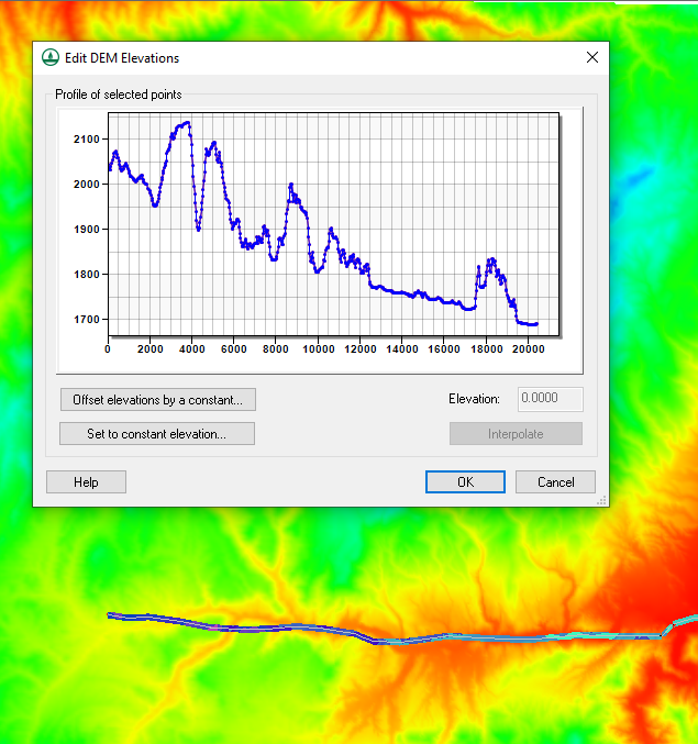
Elevation values for a TIN orDEM can be interpolated to feature objects. Doing this will add the elevation values to the feature objects, specifically to points and vertices. To interpolate to feature objects:

  1. Select the map coverage with the feature objects that will receive the elevation values to make the coverage active.
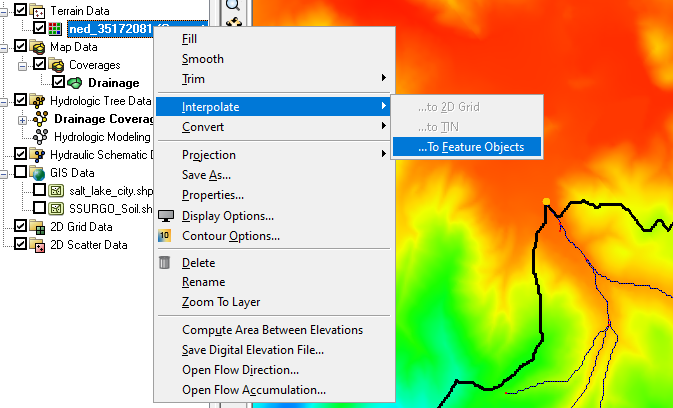
  2. In the Project Explorer, right-click on the TIN or DEM containing the elevation values and select Interpolate | To Feature Objects.
Interpolate to Feature Objects command

The elevation values on the TIN or DEM will then be added to the features objects of the active map coverage. This process will only interpolate values to the active map coverage. Inactive map coverages will not be affected and only one map coverage can receive elevation values this way.

Interpolating to feature objects uses linear interpolation. If a point or vertex lies between a DEM or TIN elevation point, the interpolation method will estimate the closest approximate value. Elevation values will not be interpolated to feature objects that are outside of the DEM or TIN area.

Typically, interpolated to feature objects is done when you have manually added features objects without designating elevation during the digitization process. It can also be used in cases where the elevation values appear inaccurate and need to be changed to match a new set of elevation values. It may also be useful after importing map data that is missing elevation data.

Try out interpolating to feature objects in WMS today!

Blog tags: 

Using the Copy to Coverage Command

In SMS, after spending time creating the perfect arc, polygon, or series of points on a map coverage, you may find that you need that feature object added to other coverages. Recreating the same feature object manually could be too time consuming. Fortunately, with the release of SMS 13.1 beta, there is now the Copy to Coverage command.

The Copy to Coverage command allows copying selected feature objects from one map coverage to another. To use the Copy to Coverage command:

  1. Create the coverage that will receive the copied feature object.
  2. Select the desired feature object or objects in a map coverage.
  3. Right-click and select the Copy to Coverage command.
  4. In the Select Coverage dialog, select the coverage that the feature object will be copied to.
Example of the copy to coverage command

When the feature object has been copied, attributes (boundary condition types, materials values, etc.) assigned to the object on the original coverage will need to be reassigned if the new coverage is of the same coverage type. Currently, feature object attributes cannot be preserved when copying to a coverage of the same type.

The Copy to Coverage command is most useful when you have a coverage with a lot of feature objects, such as those imported from a shapefile, but you are only needing one or two of those feature objects copied to a new coverage. For example, have a mesh generator coverage with arcs that would work well for boundary conditions, you could select and copy just the arcs that you intend you use as boundary condition arcs to a boundary conditions coverage. This is a faster process than duplicating the entire coverage, changing the coverage type, and deleting unnecessary objects.

You can copy multiple objects at once, by using the shift key to select multiple objects of the same type. In SMS 13.1, you can also use the universal Select Objects tool to select multiple feature objects of different types which can also then be copied to a new coverage.

Try out the Copy to Coverage command in SMS 13.1 beta today!

Blog tags: 

Batch Running MODFLOW Files

Do you have several MODFLOW simulations that you have created using GMS and would like to set all of the simulations to run overnight or over a weekend? Running a batch of MODFLOW simulations can be accomplished using a batch file. A batch file allows using the Command Prompt to run several commands in a sequence of actions. Therefore, a batch file can be used to run multiple MODFLOW simulations.

To do this, you will need to create a batch file that references the MODFLOW executable and the name file for each MODFLOW simulation you intend to run. To create a batch file, you can create the file from scratch, or you can use GMS to generate a batch file for a single simulation which can then be edited to add additional simulations.

When using GMS to create a single simulation batch file, do the following:

  1. In the Global/Basic Package dialog for the simulation, turn on the Use Custom Run Dialog option.
  2. Run the MODFLOW simulation.

Among the simulation files, you will have a *.bat file. To use this file to run multiple MODFLOW simulations, do the following:

  1. Create multiple simulations in GMS and export the MODFLOW files for each simulation.
  2. Using a text editor, open the custom run *.bat file.
  3. Edit the file include the name files for additional MODFLOW simulations.
  4. Use the Command Prompt to run the edited batch file which will then run the MODFLOW simulation sequentially.

Once the simulations have run to completion, you can load the results into GMS by creating a GMS MODFLOW results file (or MFR file) for each simulation. The file name of the MFR file should match the MODFLOW name file.The format for an MFR file can be found by examining an existing GMS MODFLOW solution set.

Example of MODFLOW results file

It is recommended that you use the GMS model check for each simulation and resolve any issues found before including the simulation in the batch run. However, if the simulation does include a problem, it will not stop the following simulations from running. In this way, MODFLOW can be run for multiple GMS projects.

Try creating a batch run for multiple MODFLOW simulations using GMS today!

Blog tags: 

Tips for Using the Hydrologic Modeling Wizard

WMS makes creating hydrologic models easier by providing the Hydrologic Modeling Wizard. This tool steps you through the process of developing a hydrologic model. Each step completes one of the elements needed for a complete hydrologic model. To make using this tool easier and more productive, here are a couple tips for using the Hydrologic Modeling Wizard in WMS.

Example of the Hydrologic Modeling Wizard

The first tip is that the Hydrologic Modeling Wizard is modular in nature. This means the wizard does not need to be closed in order to continue working in the WMS interface, unlike many other windows and dialogues in WMS. The wizard can be put to the side of your screen to let you work with other tools in WMS. Often this is necessary to adjust arcs in the Graphics Window or to import additional data. Once you are done with what you need to do, you can return to the Hydrologic Modeling Wizard.

It should also be noted that the Hydrologic Modeling Wizard keeps track of changes as you work in it. So if you should happen to close it, you can reopen it and get back to where you left off. However, you should make certain to save your WMS project before closing WMS in order to save changes made in the wizard to your WMS project.

Another tip is that you do not need to complete all of the steps in order. Some steps can be completed out of order. For example you may want to set the model you are using before completing earlier steps. Or, more often, you may have completed earlier steps outside of the wizard, letting you skip to later steps. That said, there are some steps that will not work unless a previous step has been completed.

Also note that you can always go back to earlier steps. Note that when doing this some steps that follow may have to be completed again.

The Hydrologic Modeling Wizard is a powerful tool to help you create hydrologic models faster. The tips presented here can also be applied to the other modeling wizards in WMS. Try out the Hydrologic Modeling Wizard in WMS today!

Blog tags: 

Exporting Map Data to a Shapefile

Feature objects in SMS resemble the objects in shapefiles in many ways. Shapefiles are a file format used by many GIS applications. Starting in SMS 13.1, feature objects in SMS can be directly exported into shapefiles.

SMS 13.1 allows points, arcs, and polygons to be exported from a specified map coverage to shapefile. This done by doing the following:

  1. Select the desired map coverage in the Project Explorer to make it active. It is recommended that you hide any map coverages you don’t want exported.
  2. Right-click on the coverage and select Export.
  3. In the Export Coverage dialog, select the direction where you want to save the shapefile, enter the shapefile name, and select which type of shapefile to use.
Exporting a coverage to a shapefile

Be certain to select the correct file type when exporting feature objects. Only the matching feature object type will be exported to a shapefile from the coverage. SMS allows you to export feature points as a points shapefile, feature arcs as a line shapefile, and feature polygons as a polygon shapefile.

It is also recommended to review the feature objects on the coverage before exporting to a shapefile. Individual feature objects cannot be exported at this time, therefore, it is advisable to remove any unwanted features before exported. This can be done by duplicating the map coverage and then deleting the unwanted feature objects.

If desired, you can import the exported shapefile into SMS. The shapefile will appear in the GIS module and can then be compared with the feature objects on original map coverage. Otherwise the shapefile is ready to be imported into the desired application.

It should be noted that not all data on map coverages can be exported into a shapefile format. Some data, such as boundary conditions attributes or coverage specific settings, may not end being exported.

Try out creating shapefiles from feature objects in the SMS 13.1 beta today!

Blog tags: 

Tips for Importing Wells to the Conceptual Model

In many MODFLOW projects, having the correct placement and settings for wells is important for getting correct results. GMS facilitates the implementation of wells by allowing well data to be imported directly into the conceptual model. This article gives an overview of importing well data directly into the conceptual model along with some tips.

Importing wells directly into the conceptual model first requires that the wells be in a file with the correct format. Typically this is a text file. Please refer to our wiki article for the correct format that GMS will use.

Other file formats, such as shapefiles, are also common, but often cannot be imported directly into the conceptual model. These other formats will import the wells into a different module, such as the GIS module, and will need to be converted over to the conceptual model.

Before importing well data into the conceptual model, make certain you have an existing map coverage with the well option turned on. Without this, the well data cannot be imported directly to the conceptual model.

When importing well data in a text file, you will use the Open command then the Import File Wizard. In the second step of the File Import Wizard, you must select "Well data" for the GMS data type. Also in the second step, make certain all the data columns are correctly assigned. Failing to assign the data columns correctly can result in errors.

Importing a well file into GMS

It should be noted that you are not limited to the number of data columns you have in the file. Therefore, you can import multiple wells at the same time. You can also import multiple time series or other data applicable to the wells using this method. Please note that while the wells and time series can be defined in the same text file, it is necessary to import the file twice: once to create the wells, and once to assign the time series to the wells. Constant flow rates can be imported at the time of well creation.

Review the well data after it has been imported. That can be done quickly by bringing up the coverage attribute table dialog for the wells. If the data was not imported correctly, minor changes can be made in using the tools in GMS.

Try out importing well data directly into the conceptual model using GMS today!

Blog tags: 

Converting Soil Data to an Index Map

Do you need to add soil data to your GSSHA model in WMS? Soil data is often needed in a rainfall/runoff GSSHA model so that infiltration can be considered in the model. WMS makes this easy by allowing soil data to be converted to an index map.

In order to include soil data in your GSSHA model, there are few steps to follow.

First, you will need a soil data map coverage. Once this coverage has been created you can add soil data directly to the map coverage. Often, you may have soil data located on a shapefile or other source. The soil data on the shapefile needs to be mapped over to the soil data coverage before creating the index map.

Second, the index map will be included with a 2D grid for the GSSHA model in WMS. Make certain you have created your 2D grid and initiated your GSSHA model.

Finally, convert the soil data coverage to be an index map in your GSSHA project. This is done by doing the following:

  1. Use the GSSHA | Maps command.
  2. In the GSSHA Maps dialog, set the soil data coverage to be used.
  3. Click the Coverages to Index Map button.
Soil data converted to an index map

Once you have converted your soil data to an index map, you can use it in your GSSHA model.

When converting soil data to an index map, we do have some tips to make it go smoother.

  • When converting a shapefile to a soil data coverage, make certain that the soil data with the shapefile has been joined to the shapefile.
  • After mapping a shapefile to a soil data coverage, make certain that the soil data mapped over.
  • Check to see if soil covers the entire area of the 2D grid. A warning may appear if the soil data does not cover the area of the 2D grid.

Once your soil data have been successfully converted to an index map, it is ready to be used in your GSSHA model.

Try out using soil data with GSSHA in WMS today!

Blog tags: 

New Map Annotation Tools in SMS 13.1

With the release of SMS 13.1 beta, a new tool has been added to allow you to have additional annotations on feature objects. SMS already provides several options for adjusting how feature objects are displayed, but now more options exist specifically for feature arcs to help make working with feature arcs easier.

Currently in recent versions of SMS, annotations can be added to label arcs. This would let you see the name of specific arcs. The color and thickness of feature arcs can also be changed. Also, specific annotation options exist for specific model coverages, such as the SRH-2D boundary conditions map coverage.

The new map annotations can add a number of new annotations to your feature arcs.With the new annotation tools, the following can also be displayed:

  • An arrow indicating the the direction of the feature arc
  • Tick marks to indicate the distances along the arc
  • The length and number of tick marks can be adjusted along the arc
  • Tick mark labels can be added
  • The font and color of tick mark labels can be changed
Map module annotations in SMS 13.1

These options allow you to quickly see if an arc has been placed in the wrong direction or to check the measurement of an arc. Note that tick marks will use the units set in the project's projection.

To activate the map annotations, do the following:

  1. Open the Map Display Options
  2. Turn on the Annotations option under the Arcs section
  3. Click the Options button next to the Annotations option
  4. Turn on the different the map annotations options in the Arc Annotations Options dialog

Note, with the exception of the tick mark color, that the line width and color are still determined by the other arc display options. The display of the arcs can be adjusted before or after setting the arc annotation options.

Try out the different map annotation options in the SMS 13.1 beta today!

Blog tags: 

Using the SAMG Solver for MODFLOW

Are you needing to use multiple processors to run your MODFLOW or MODFLOW-USG model? Using multiple processors can speed up the model processing time. In order to use multiple processors for MODFLOW in GMS, the SAMG solver provides the means to do this.

The SAMG solver is developed by the Fraunhofer Institute for Algorithms and Scientific Computing (SCAI). It contains a library of subroutines for the highly efficient solution of large linear systems of equations with sparse matrices. SAMG has an advantage in being almost unconditionally numerically scalable. This means that the computational cost using SAMG depends linearly on the number of unknowns.

Before using the SAMG solver, check to see if you have it added to your license. Do this by going to the Register command in the Help menu. Look through the list of components to make certain the SAMG parallel interface / solver has been enabled.

The SAMG solver works with the LMG solver package in MODFLOW. The LMG solver needs to be selected to access the SAMG solver. The LMG solver links the MODFLOW project to the SAMG solver.

SAMG warning message

To activate the SAMG solver do the following:

  1. Open the MODLOW Global/Basic Package dialog.
  2. Then open the MODFLOW Packages dialog.
  3. Turn on the LMG – Link-AMG option.
  4. A warning may appear discussing the SAMG solver. This warning can be turned off if desired.
  5. Once the LMG solver has been turned on, the Link-AMG (LMG) Package dialog can be accessed through the MODFLOW menu in order to set the solver parameters.

Using the SAMG solver is not ideal for all MODFLOW projects. It is generally meant for large linear problems and simulations which use several time steps. For the right project, SAMG can help significantly accelerate the model run time.

For MODFLOW-USG, the SAMG solver is used with the SMS Solver. You can select the SAMG solver in the SMS Solver options.

Contact Aquaveo's licensing team to see about using the SAMG solver with your GMS projects.

Blog tags: 

Editing DEM Elevations

Do you have a Digital Elevation Model (DEM) that has elevations that need to be adjusted? Editing DEM elevations can sometimes prove difficult. However, with WMS you can edit the elevations of DEM files using several tools WMS provides for editing DEM elevations.

Here are a couple ways DEM elevations can be edited in WMS:

Editing Single Points

Some DEMs have a single point where the elevation is off. You can edit a single point in a DEM by using the Select DEM Points tool and selecting the point. You can then edit the point elevation by double-clicking on the point to bring up the DEM Point Attributes dialog where the elevation value can be changed.

Using Feature Arcs to Edit Elevation

Sometimes, the elevation of a DEM needs to be adjusted to follow a specific line, such as a river bed or proposed irrigation channel. The elevation in this location can be adjusted using a feature arc. This is done by selecting the feature arc then right-clicking and selecting the Edit DEM Elevations command.

Editing DEM Elevation using an Arc

In the Edit DEM Elevations dialog, you can change the elevation of the DEM along the arc. This can be done by selecting and changing elevation points on the arc in the profile window. For editing all of the elevation values along the arc, the dialog provides the following options:

  • You can offset all of the arc elevations by using the Offset elevations by a constant button.
  • You can set all of the elevation values to a constant by using the Set to constant elevation button.
  • Finally, you can use the Interpolate button to interpolate the values to between the first and last values on the arc. This will smooth out the elevation to create an artificial slope.

Using these tools makes adjusting the elevations of DEMs easier. Try them out in WMS today!

Blog tags: 

Pages