Aquaveo & Water Resources Engineering News

Using the Temporal Tools in the Dataset Toolbox

SMS contains several ways to work with datasets. Perhaps the most useful of these is the Dataset Toolbox. The Dataset Toolbox has several tools for generating new datasets. Among these are the temporal tools which allow adjusting the time steps for a transient dataset. The temporal tools include two options: Sample Time Steps and Merge Dataset.

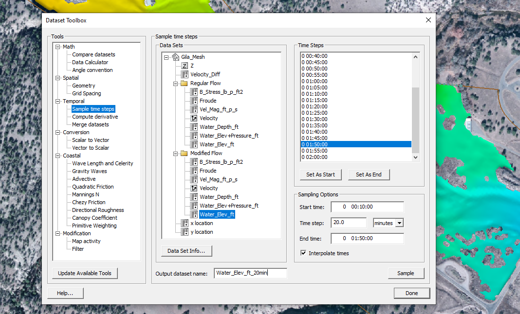
The Sample Time Steps tool allows the creation of a dataset with a different number of time steps. The time steps can either be increased or decreased. To use the Sample Time Steps tool:

  1. Open the Dataset Toolbox and select the Sample Time Steps tool.
  2. Select the transient dataset you want to use.
  3. Select the starting and end times.
  4. Enter the time step frequency and units.
  5. Give the new dataset a name and click Sample.
Dataset Toolbox showing the Sample Time Steps tool

The other temporal tool is the Merge Dataset tool. This allows us to combine two transient datasets. To use this tool, the transient datasets being combined cannot have overlapping time steps. Most often, this tool is used to append multiple simulation runs together.

For example, if you completed an SRH-2D model run for one day, then created a new simulation for a second day (using a hot start file from the end of the first day simulation run), you could combine the results of the two simulation runs using the Merge Dataset tool.

To use the Merge Dataset tool:

  1. Open the Dataset Toolbox and select the Merge Datasets tool.
  2. Select the first dataset to use, then select the second dataset.
  3. Enter a name for the combined dataset and click Compute.

When using the Merge Dataset tool, make certain that the first dataset selected has time steps that are earlier than the second dataset selected.

The temporal tools in the Dataset Toolbox provide a simple way to adjust transient datasets in your project. Try using these tools in SMS today!

Blog tags: 

The HDF5 File Format and MODFLOW

The HDF5 file format is a cross platform binary format for storing scientific data. HDF5 allows you to reduce the size of the file data by compressing repeated values. This allows your data to be read and written much faster than if you stored the data as ASCII (plain text) files. GMS can read and write to HDF5 files, and stores its own HDF5 files with the other MODFLOW data files.

Exporting an HDF5 file

There are no hard file size limits. The number of objects within an HDF5 file is not limited, and the format supports complex relationships through grouping and linking. In addition to support for common metadata types, you can create user-defined metadata to accommodate whatever needs you have in your project. The only limits with these are the capabilities of your computer.

HDF5 was designed to be extensible and to allow for future changes to the platform. GMS takes advantage of this by checking HDF5 data for key values in order to substitute them into your arrays or lists. This allows you to better use transient parameters and very large pilot point sets. GMS handles the pilot point interpolation through an external routine that helps speed up the processing.

There are external HDF5 file viewers and editors, such as HDFView. However, it is very easy for you to modify the data in such a way that it makes the HDF5 unreadable by GMS. Because of this, we recommend only viewing the files using these tools. You should only manually edit the file if given explicit directions by a developer. If modifications need to be made to the HDF5 file, we recommend you make the changes to your project in GMS which will re-export the HDF5 file.

Learn more about the HDF5 file format from the HDF Group, a consortium of scientists worldwide that works on the HDF5 format. You can also read the article on the XMSWiki about using the HDF5 format with MODFLOW. This article goes into more details about multiple specific uses for the file format.

Make use of HDF5 files with MODFLOW in GMS today!

Blog tags: 

Using Pre-Generated Polygons to Delineate a Basin

Delineating an accurate basin is an important part of a watershed project. WMS provides a number of tools for delineating a watershed basin. The Hydrologic Modeling Wizard is often used to step through the entire process of delineating a basin.

However, it is possible to delineate a basin using data from outside of the Hydrologic Modeling Wizard. In particular, the Drainage module contains tools for delineating a basin using existing project data.

For example, if you have a shapefile with polygons that gives the general outline of the basin, that shapefile can be used to delineate the basin. To use the shapefile polygons to delineate the basin, do the following:

  1. Import the shapefile into WMS. Verify the location is correct.
  2. If you have not already done so, add a DEM for the area of interest to the project.
  3. Generate the flow direction and accumulation, either by running TOPAZ/TauDEM or by importing it.
  4. Map the shapefile polygon(s) into feature polygons in a drainage type coverage.
  5. Place your outlet point(s) and digitize the streams. You can either manually draw the arcs, or load the streams from a shapefile. Be sure to verify that the arcs are set to Stream (not Generic) and that the directions are flowing from upstream to downstream (see "Stream Arrows" in the Drainage Display Options).
  6. Select DEM | Polygon Basin IDs -> DEM in the Drainage module.
  7. Select DEM | Compute Basin Data in the Drainage module.
Basin delineated from shapefile

Once you have a delineated basin, you can use the basin with the watershed modeling model of your choice. Be certain to review the basin to make certain it contains all of the area you need for your project.

WMS provides a large amount of flexibility in delineating a watershed basin in order to adapt to the needs of your project. Try out the different basin delineation tools in WMS today!

Blog tags: 

Viewing Vectors on the Watersurface

With the release of SMS 13.1 beta, a new option has been added to the Vector tab. The existing Vector tab in the Display Options dialog allows viewing vector data as arrows as data points in your project. SMS can change the density of how the vector arrows are displayed and to display the vector arrows along a constant elevation. This new option allows you to display the model vectors relative to a selected dataset.

To use this option:

  1. Open the Display Options, turn on vectors, and go to the Vector tab.
  2. On the Vector tab and change the Origin to be "Relative to dataset".
  3. Select the Dataset button under the Origin to bring a tree item selector dialog.
  4. Select the Dataset you want to use.

After closing out the Display Options dialog, you will be able to see the vectors relative to the selected dataset. For example, if you use a water surface elevation dataset, you would be able to see the vectors relative to the water surface elevation.

Vectors relative to the water surface elevation

This option is available for all modules that allow displaying vectors. This includes the 2D mesh module, Cartesian grid module, quadtree module, and scatter set module.

There is also an option to specify an offset for the selected dataset. For example, you could set the offset to 1 or 2 to get the vectors slightly above the surface. The result would show the vectors mapped 1 or 2 feet above the ground elevation.

Vectors offset from ground elevation

This addition to the vector display option can be used with any dataset in the same module. Therefore, any dataset in the mesh module can be used with a mesh, any dataset in the scatter module can be used with a scatter set, etc.

Try out using the new "Relative to dataset" vector display option in the SMS 13.1 beta today!

Blog tags: 

Using the CLN Package to Model Faults and Fractures

Needing to model features or faults in your MODFLOW-USG model? The CLN Package is used in conjunction with MODFLOW-USG to model features that are significantly smaller than the individual cells in a 3D groundwater flow model. This tool allows you to model one-dimensional linear features within a three-dimensional simulation domain when the flow connections are separate from those of the aquifer. This makes it ideal for modeling fractures and faults.

CLN network map

There are a number of requirements to use the CLN package:

  1. The MODFLOW version must be set to MODFLOW-USG in the MODFLOW Global/Basic Package dialog.
  2. There must be a coverage with Wells and Wells (CLN) turned on in the Coverage Setup dialog.
  3. The coverage must have a default layer range of at least two layers, and it must be active on the layers where the CLN features will be.

The CLN package works with unstructured and 3D grids. It allows connections to be set up between the CLN cells to regular groundwater cells. You can connect a CLN cell to one or more groundwater flow cell, and CLN cells do not have to be ordered upstream to downstream. These features allow you to scale the conceptualization of the flow as needed.

For example, a single cylindrical CLN cell (representing a long fracture or fault within the ground) connected to multiple groundwater flow cells may be pumped to simulate multi-node well connections. The CLN cell extracts water from the groundwater flow cells as part of the solution to the coupled CLN and groundwater flow equations.

You can treat a CLN cell as a well by using the WEL Package to assign a source or sink to the cell. This can also be done using multiple CLN cells. Multiple fractures can be connected together to form one larger network. To make things easier, you can also use shapefiles to map the features of the CLN cells and connections.

CLN network map examples

By using this method, you can create a more complete picture of the domain you are modeling. Try using the CLN package to model faults and features in GMS today!

Blog tags: 

Troubleshooting TOPAZ and TauDEM in WMS

Both TOPAZ and TauDEM make computing flow directions and accumulations for basin delineation easier. One of these two programs is typically used during the process of delineating a watershed. During this process, it is not unusual to run into some issues. Below are some common issues and how to resolve them.

Missing DEM

DEM data is required to run TOPAZ or TauDEM. A DEM can be imported from a file or downloaded from a web service. If you get an error stating that no DEM exists after you have imported the DEM data, this is typically because the DEM was not imported correctly.

TOPAZ unable to find DEM

Often, the DEM has been imported as a raster file and is in the GIS data module. In order for TOPAZ or TauDEM to use this as a DEM it will need to be converted from a raster to a DEM using the Convert to | DEM right-click command in the GIS module.

Not Enough Data

In order for TOPAZ or TauDEM to work properly, a DEM is needed that has enough data to work with. When working on modeling very small areas, TOPAZ or TauDEM may fail to execute correctly because there is not enough data available to complete the process.

In order to fix this issue, it is recommended that you slightly expand the size of the area you are modeling. In particular, the resolution of the DEM being used may need to be increased. Use your best judgement as to how much additional data to add.

Too Much Data

The opposite of having too little data would be to have too much data which causes TOPAZ or TauDEM to slow down or stop running altogether. This typically happens when attempting to model a very large watershed. In this case, the issue typically isn’t related to problems with TOPAZ or TauDEM but is more likely related to the available processing power of the computer being used.

With many projects that have too much data, often much of that data is unnecessary. Often a lower resolution DEM can be used. When modeling a large watershed area, you should use your engineering judgement to find areas of greatest interest and then focus on those areas. If that is not possible, then you will need to find a way to increase your computer's processing power.

TOPAZ and TauDEM tools for delineating a basin. Try them out in WMS today!

Blog tags: 

Announcing SMS13.1 Beta

Aquaveo is pleased to announce the release of SMS 13.1 Beta! A number of new features have been added to this version, and we'd like to highlight a few of them.

3D Bridge

The new 3D Bridge feature allows creating a visual representation of a 3 bridge. This representation uses a 3D UGrid to visualize the bridge in the graphics window. After creating a 3D bridge, the feature can be visualized in an observation profile plot.Using the 3D feature allows generating a ceiling elevation dataset to represent the maximum water surface that can be reached at each point in the mesh at the intere. The bridge data can be exported as an XMUGRID file for use in multiple projects.

3D bridge example in SMS
Universal Select Tool

The Select Objects tool allows selecting multiple types of feature objects at the same time from the same tool. The selection information at the bottom of the screen changes if multiple types of objects are selected to show how many of each object is selected. The right-click menu changes to match the selected object type. If multiple feature object types are selected, then the right-click menus will be combined.

Extract Features

The Extract Features tool allows you to use a raster to generate feature arcs for channel centerlines, ridge centerlines, or channel cross sections and banklines. This can speed up the creation of the centerlines and cross sections by removing the need to manually create each feature individually. Options for this feature include the ability to extract all centerlines, extract all centerlines with one or more selected depression points, extracting a single centerline, or extracting channel banklines and cross sections.

Example of extracted feature arcs
HEC-RAS 1D

SMS 13.1 Beta includes support for creating and editing HEC-RAS 1D cross sections and attributes. These cross sections can be imported from HEC-RAS as SDF files and saved as a HEC-GeoRAS file for inclusion into a HEC-RAS project.

These are just a few of the new features in the SMS 13.1 beta. Try out these features and more by downloading the SMS 13.1 Beta today!

Blog tags: 

Using MODFLOW-NWT for Mine Dewatering

Have you tried dewatering a mine model using MODFLOW-NWT? MODFLOW-NWT is a version of MODFLOW provided by the USGS that uses a method to solve MODFLOW models that are non-linear due to unconfined cells or non-linear boundary conditions, creating an asymmetric results matrix. Because mines that need to be dewatered sit below the water table, cells within the simulation will become dry at times due to the removal of the water from the mine. MODFLOW-NWT is great for such situations as it handles dry cells well.

Modeled mine example

Mine dewatering models are often used when estimating the required flow capacity for the pumps used in the field. You can create a regional model to establish a baseline, then create one or more models with various pit depths to establish the best approach for the mine in question. While elevations cannot be set to transition during a MODFLOW run, multiple conceptual models can be created within the same project in order to keep all of the data together.

It’s important to remember the difference between wells and drains when creating the dewatering model. Drains only subtract water when the head is above the elevation of the drain. Therefore, drains can be used to represent the seepage face around the edges of the pit, and the drain elevations should be set to equal the ground surface elevations. The amount of water removed by a drain is related to the conductance of the material of the seepage face. Drains are generally used at the bottom and side seepage faces of the mine.

Wells remove a specific amount of flow, and can therefore dewater the cell they are in prior to dewatering the rest of the mine. MODFLOW-NWT, as mentioned previously, handles these dry cells very well, keeping them active in case they become wet again.

Because MODFLOW-NWT uses 3D grids, you should make sure the cells inside the pits are inactive. You do this by creating the boundary polygon, and then removing a "donut hole" of cells within the pit area. Use the Activate Cell(s) in Coverages tool to inactivate the cells. You’ll have to do this for each layer, and each layer should be on its own coverage.

Finally, always use the Model Check to make sure there aren't any obvious errors or missing values in any of the inputs. After MODFLOW-NWT finishes running, you should review the water table by looking at the drawdown output contours. You can also do this by switching to Ortho view and reviewing the head in the appropriate rows or columns.

Try out making a mine dewatering model using MODFLOW-NWT in GMS today!

Blog tags: 

Using Plots in CityWater

Any presentation about water distribution management can be improved with the right plots. CityWater has a number of different plots accessible through the plot icon on the Map View page that can be used by you to visualize the information available in each of your projects. These plots can be used in reports or presentations to help others understand details and specific time-based information you need to share.

The Plot icon on the Map view is a dynamic tool. If no nodes or links are selected, it will display a System Flow Balance plot when clicked. This plot shows the flow produced, consumed, and stored within your pipe network. You can select any point along each of the plot lines to see specific for that time.

CityWater System Flow Balance Flow

If you have a specific link or node selected (or more than one of either nodes or links selected), you can use the Layers tab drop-downs to select what will appear on the plot. This gives you a large number of possibilities for how the plot will appear. Some combinations do not have a plot available, and these will instead show the default System Flow Balance plot. We recommend taking the time to play around with the options to find the ones that will work best for you.

For example, the image below shows a plot with Demand, Links, and Minimum selected from the Node Layer, Link Layer, and Time drop-downs (respectively). As before, you can select any point along the plots to see specific details for the desired node or link.

CityWater Demand Plot

CityWater contains many other tools to help you visualize water flow and usage in your water distribution network all in an accessible and a convenient to use web environment. Learn more about how CityWater can help your organization today!

Blog tags: 

How SRH-2D and HY-8 Work Together

SMS allows using HY-8 to create culverts in SRH-2D models. HY-8 was created to model culvert profiles. When SRH-2D was being developed, structure boundary conditions were allowed to be linked HY-8 culverts to SRH-2D. Doing this permits SMS to make use of the more robust tools of HY-8 when designing culverts.

When designing a culvert for an SRH-2D model in SMS 13.0:

  1. Right-click on the SRH-2D BC coverage and open the HY-8 Options dialog.
  2. From the dialog, create the HY-8 file for the project.
  3. On the SRH-2D BC coverage, create two arcs for the culvert: one for the inlet side of the culvert and one for the outlet side.
  4. Select both arcs and open the SRH-2D Linear BC dialog.
  5. In the dialog, select the Culvert HY-8 option and launch HY-8 to connect the HY-8 file.
  6. In HY-8 design your culvert.
HY-8 with SRH-2D

There are a few items to keep in mind when creating your culvert:

  • Pay attention to where the culvert is located and how it snaps to the mesh in SMS. Designing your culvert for a location that doesn’t match up with your culvert is designed in HY-8 can cause discrepancies. Also, it helps to have the inflow entering the culvert at as close to a 90 degree angle as possible.
  • Note that the crest length for constant elevation roadway profiles is the length between embankments.
  • After the initial model run, the inflow values to the culvert may need to be adjusted and calibrated. If SRH-2D is showing lower or higher flow values, adjust the values in HY-8 as needed.
  • Using a monitor line at the inlet or outlet side of the culvert. The results of the monitor lines may be different than what HY-8 reports. Use this difference to calibrate the model.
  • 2D mesh elements are disabled between the culvert arcs during the model run.

HY-8 makes a great addition to SRH-2D in SMS. HY-8 is shipped with SMS, so feel free to try it out with your models today!

Blog tags: 

Pages