Aquaveo & Water Resources Engineering News

Viewing an Aquifer's Water Level

After completing a MODFLOW groundwater model in GMS, have you needed to see the aquifer water level? Viewing the water level can aid in visualizing the saturated thickness of an aquifer. The water level can be viewed by doing the following:

  1. Ensure that the Ortho Mode option is toggled on.
  2. Go to Display | Display Options, choose 3D Grid Data, and go to the MODFLOW tab.
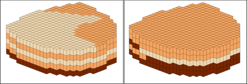
  3. Toggle on the Water Table option, and click OK.
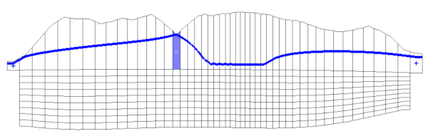
  4. Choose either the Front View or the Side View option, or select a cross section to view the water table level.
Water Table shown in GMS

Additional information about the MODFLOW display options, including the Water Table option, can be found on our wiki.

After viewing the water table, it is possible to save the spatial 2D data for the saturated thickness (water table thickness from the aquifer base).

There isn't a shortcut way to save the 2D water table thickness. However, the desired dataset can be created by converting the head and bottom elevation datasets to 2D datasets, and using the dataset calculator to create a dataset of the difference between the two datasets. The workflow is outlined below.

  1. Right-click on your 3D grid and select Convert To | 2D grid.
  2. Select your Head 3D dataset.
  3. Go to the Grid menu, and select 3D data → 2D data.
  4. Choose the desired option in the Create dataset using dialog box selecting the option that best fits your desired dataset.
  5. Repeat steps 2–3 for the Bottom MODFLOW dataset.
  6. Select the 2D grid and go to Edit | Dataset Calculator.
  7. Create the expression: head dataset minus bottom dataset.
  8. Note: If you would like to create a dataset of all time steps, check the box next to Use all time steps before computing.
  9. Give the new dataset a name in the Result option, and click Compute.
  10. Your new dataset will appear under the 2D grid.

Now that you know how to view and save a water table, try it out in GMS today!

Blog tags: 

Bringing Water Stability to the World

A project that Aquaveo is proud to be part of is bringing forecasting data to people around the globe through GEOGLOWS.

Because many countries around the world don’t have the resources to predict droughts and floods, they struggle to keep a steady supply of food and stable economy. Companies such as the World Bank, ESRI, NASA and others have partnered together to create a warehouse of apps to predict a 15-day forecast of more than 200,000 streams across four continents to help anyone from farmers to politicians be better prepared for any changes.

GEOGLOWS workflow

Though Aquaveo only came onto this project recently, designing an API for these apps, we are very excited to be helping countries around the world such as Somalia and Ethiopia overcome their struggles to stabilize their economies, and be better prepared for disasters.

Two of Somalia’s main rivers, the Juba and Shebelle rivers, originate outside of their boundaries in Ethiopia and Kenya, which is a major obstacle for Somalia. A streamflow forecasting system helps improve water management in the country by providing much needed transboundary water information--helping them foresee flooding within days allowing them to take action.

Ethiopia gets between 40–87 inches of rain a year, both because of this much rainfall and in spite of this much rain, Ethiopia is vulnerable to floods, droughts, and chronic scarcity in several parts of the country. A streamflow forecasting system helps improve water management in the country by providing the necessary data to make decisions and develop action plans.

Since the formal creation of the initiative in 2017, the most significant element of GEOGLOWS has been the application of Earth Observations (EO) to create a system that forecasts flow on every river of the world while also providing a 35-year simulated historical flow. We can now deliver reliable forecast information as a service, instead of all the underlying data that must be synthesized and computed locally to produce the necessary information.

Aquaveo have been proud to be part of GEOGLOWS and other initiatives. Watch our website to see news about more projects like this in the future.

Blog tags: 

Best Practices for 2D Hydraulic Modeling

In SMS, designing a good 2D hydraulic model from the start gives the best results. A poorly designed model can give bad results, cause model errors, or even keep the model from converging. And while it may seem easy at first to design a good model, there are plenty of potential pitfalls that can come up if you are not careful.

The following tips, broken down into five areas, can help improve any model.

Terrain Data

Pay attention to your terrain data. You can't set up a good model without a good foundation, and terrain data is your foundation. There are four things you will need to spend time getting right:

  • Represent hydraulic controls accurately
  • Make sure you include channel bathymetry
  • Add breaklines where needed
  • Finally review the terrain surface for missing features
Terrain review
Mesh Development

Use an appropriate number of elements: size does matter, more is not always better. This is mainly because the time your model takes to render is a significant factor for any project. Element length should generally be equal to or greater than the flow depth, except for limited areas such as piers. When elements are too small, waves can form skewing the model results.

Quadrilatereal elements in meshes are often more stable than when using triangular elements. Once you have set your number of elements and length, confirm that hydraulic controls are represented in the mesh.

Lastly, review your mesh for quality.

Mesh quality review
Boundary Conditions

When determining the boundaries of your model, you will need to find two things. First look for the most constricted area when determining model limits. Second, find the furthest usable boundary location from the area of interest. A good rule of thumb for rivers: two floodplain widths up and downstream. Note that the width of the mesh should be greater than the maximum flood width.

Lastly, perform sensitivity analysis on boundary conditions.

Material Roughness

Be aware that Manning's n values for 2D model can be lower than 1D models. Be sure to calibrate your model. Essentially check your results to see if they are reasonable.

Model Execution and Review
  • Use the largest time step possible that gives you continuity and stability ( i.e. while still achieving a good solution).
  • Use monitoring points to verify steady simulation.
  • Use monitoring lines to verify continuity.
  • Review convergence parameters to confirm conservation of mass.

Following these tips can improve any model that uses a 2D mesh. Try them out in SMS today!

Blog tags: 

Tips for Flow Budget in GMS

In any groundwater model, knowing how much of the groundwater is available for use determines the fate of any project planned for the area. It is often a crucial part of a model to determine an accurate water budget or flow budget. MODFLOW can calculate its own flow budget and can also make use of the ZONEBUDGET program to calculate the water budget for subregions of a model. Knowing how to use both the MODFLOW flow budget and the ZONEBUDGET program greatly enhances the value of models built in GMS.

PZONEBUDGET example

With that in mind, here are some tips for making use of a flow budget and ZONEBUDGET in GMS:

  • If ZONEBUDGET is used to calculate a budget for the entire modeled area, the values for each budget term should match the MODFLOW budget except in situations where there are multiple stresses of the same kind in the same cell (e.g. a pumping well and a recharging well in the same cell).
  • You can confirm your approach by calculating the cumulative volumes for the entire model and seeing if they match the MODFLOW outputs.
  • Computer precision could be a cause of small discrepancies between the budgets produced by ZONEBUDGET and MODFLOW. ZONEBUDGET accumulates budget totals using double precision, and MODFLOW uses single precision. Because of the use of double precision, ZONEBUDGET's output should generally be more accurate than MODFLOW's; however, differences in output are not likely to be significant except for some very large models.
  • You can find the correct cumulative volume of water entering a given zone using the flow rate. This is done by multiplying the rate by the length of the corresponding time step.
  • Rates reported are for the same duration of the matching time step. Time steps stair step, so there the value is the same for the entire time step.

For an overview of ZONEBUDGET in GMS, see our tutorial and try it out in GMS today!

Blog tags: 

Working with Large DEMs

Do you have a project that requires using a large DEM? Digital Elevation Model files are a great source for terrain data in WMS. A lot of projects require using DEMs which makes it important to use the data available.

Using a large DEM file can present some complications in WMS. A large file may cause the program to slow down or have difficulty processing. So it is important to make certain to use a DEM that contains mostly relevant data and doesn’t contain an excess of nonessential information.

But how do you know if the DEM data you are pulling is enough? Is more watershed data always better?

Example of DEM in WMS with contours turned on.

Pulling in more data doesn’t insure better results. Though WMS is able to handle a massive amount of data (which is not a guarantee) the hardware in your computer may not be able to handle it. In general, a DEM twice the size of your watershed is probably sufficient for most models. More than twice your watershed size tends to just bog down the model causing you to face unnecessary wait times.

What should you do if your watershed data is not loading?

If your data is taking a long time to load try adjusting the resolution. After using the Get Data from Map tool, and making your selection in the Data Service Options dialog, you will be able to select your desired resolution in the Zoom dialog. Selecting a lower resolution zoom level should make the DEM easier to work with in WMS.

You could also try breaking up the DEM into multiple DEMs. That way your computer is not overwhelmed by trying to download one huge file all at once. Then while you’re working on your model you can turn on just the DEM(s) you need.

Third party software can be used to break up the DEM or reduce the resolution.

DEMs remain an excellent source for data for projects in WMS. Download WMS today!

Blog tags: 

Using the Prune Arc Tool

The Prune Arc tool is relatively new to SMS, and we're excited to show you just how useful it can be.

The Prune Arc tool is similar to the smooth arc function in SMS. This Smooth Arc tool is useful when eliminating noise from a rough arc, and can make your variations more mathematically stable. This can be extremely handy in working with a model—especially in situations like coastal modelling, which are prone to busy edges. Unfortunately, smoothing an arc can also change the shape of the arc to the point where it no longer matches the actual coastline.

You may come across a situation where your imported arcs have a lot of unnecessary roughness or concave areas that you want to eliminate without redistributing your vertices along the rest of the arc.

If this is the case, the Prune Arcs function is just the tool for the job. This tool trims—or prunes—rough edges and outlying spikes without rounding or reshaping the rest of the arc. Specifically, it allows you to focus on smoothing one side of the arc. This is helpful in coastal modeling where there may be a small river mouth, a harbor, cove or other concave sections that you do not want to include in your model.

Prune arc example

Access the Prune Arc tool by doing the following:

  1. Use the Select Feature Arcs tool to choose the arc or arcs you wish to prune.
  2. Right-click on the selected arcs then, in the menu, select the Prune Arc(s) command.

This will bring up the Prune Arcs dialog box, from which you can choose your pruning settings.

There are two types of pruning that can be done: Constant and Spatially Varying.

  • Constant will prune everything within a specific measurement set by you. This measurement is in meters by default. The larger the number, the more dramatic the pruning will be.
  • Spatially Varying uses the numbers in a particular dataset to establish the parameters of the pruning. This dataset is chosen in the Prune Arcs dialog box.

Importantly, you must choose which side of the arc to prune. The sides of the arc are determined by the arc direction. So if the arc is moving south to north, the left side of the arc will be on the left side of your screen. If the arc is moving west to east, the left side with be towards the top of your screen. Make certain you are pruning the correct side of the arc.

Try out using the Prune Arc tool in SMS 13.0 today!

Blog tags: 

Tips for Using Multiple Conceptual Models

Have you ever built a model in GMS that uses multiple conceptual models? Doing this offers a few advantages. However, there are potential pitfalls as well when doing this. We will discuss some of the advantages in using multiple conceptual models and what to watch out for.

A conceptual model may contain one or more map coverages. Each coverage should contain feature objects defining key structures of the groundwater model, such as wells, rivers, or recharge. Everything in the conceptual model can then be mapped over to a grid or MODFLOW model.

Example of multiple conceptual models in the Project Explorer

Beyond using folders under a single conceptual model, one of the main advantages with using multiple conceptual models is for organization. When wanting to make variations on a model, it is helpful to have one base conceptual model and then multiple variant conceptual models. The entire base conceptual model may be duplicated to provide a starting point for other variations, or individual coverages may be duplicated and dragged to other conceptual models. Duplicating the base conceptual model can be particularly helpful if you already have transport species defined for MODFLOW-related models.

For example, you can use one conceptual model for a base steady-state model, then create another conceptual model for a transient predictive model. With this you can map the base conceptual model to MODFLOW and run that model. After you have the base results, you can duplicate the solution datasets to preserve them, adjust Global Options—such as Stress Periods—if needed, and then map the predictive model to the grid to run your second MODFLOW model.

When using multiple conceptual models, there are few items to look out for. These include:

  • When changing the conceptual model, changes are not automatically made to the MODFLOW model or other models being used. The conceptual model must be mapped over to the groundwater model in order for the defined features to be included in the model run.
  • When mapping over the conceptual model, it will overwrite any existing data in the same packages contained in the conceptual model. If you want to update the model with the new conceptual model, this is the correct workflow. However, if the original conceptual model used packages that are no longer used in the new conceptual model, then there could be an error in the model run. Always review your model after mapping to confirm the features mapped as you intended.
  • When using MODFLOW-USG, and you have multiple UGrids, make certain the conceptual model is mapping to the correct UGrid or model. It will map to the active UGrid.

Working with multiple conceptual models can expand your options for your model. Try out the conceptual model and other features of GMS today!

Blog tags: 

Converting a 2D Scatter to a Raster

Have you ever needed to convert a 2D scatter set to a raster? A new feature of SMS 13.0 allows converting a 2D scatter set to a raster from the right-click menu in the Project Explorer.

Being able to convert from a 2D scatter set to a raster is particularly useful when collaborating with a colleague, or switching between programs. There are many types of raster files that can be shared between different applications.

To convert a 2D Scatter right-click on the 2D Scatter Set under Scatter Data folder in the Project Explorer and go to Convert | Scatter → Raster.

In the Interpolate to Raster dialog you have three options for Interpolation:

  • Linear
  • Inverse Distance Weighted
  • Natural Neighbor

Each option for interpolation is slightly different from the other focusing more on lower z values, higher z values, or the x and y values. Feel free to compare all three with your 2D scatter set.

Once you have selected the interpolation type you can choose to truncate some of the data by clicking on the Options button to launch the Interpolate dialog. Using the truncating option removes data from your raster. Some scenarios many only be visible in Plan view.

When you have selected your interpolation method, and truncation value if you so desire, then selecting OK will direct you to saving your raster file. You have two file type options:

  • Geo TIFF Tiles (*.tif)
  • Arch Info ASCII Grid Files (*.asc)

If you select the ASCII file type you may be asked to select a global projection, whereas the TIFF option does not. By default the raster will be imported into your current project.

When converting a scatter set to a raster the program may need to make some adjustments to outlying points. With each of the interpolation options, SMS adjusts the data for slightly different raster results.

You can see that the converted raster closely reflects the original dataset. The scale on the left of the Graphic Window will show you how closely the two are alike.

2D raster to scatter example

Now that you know how easy it is to convert a 2D scatter set to a raster try it in SMS today!

Blog tags: 

Aquaveo User Conference 2019

The 2019 Aquaveo User Conference is going on now. It started yesterday, October 8th, and will wrap up today, October 9th. We are enjoying meeting with users from around the world. In attendance are users from the United States, Germany, Portugal, South Africa, and other places around the globe.

At the conference, we announced some of the new features and upcoming changes to our products that we are excited about:

  • Making XMS functionality available for use outside of the traditional interface.
  • More web-based applications for portability and ease of access.
  • Simplifying and unifying tools so it is easier to find and use the functionalities available.
  • Project management tools to track the history of a model.
  • 3D bridge modeling in SMS.
2019 Aquaveo User Conference

Talking to those in attendance, we learned they enjoyed:

  • Learning more about software features and functionality.
  • Learning how to improve their model development process.
  • Discovering benefits of Aquaveo’s software over other software.
  • Talking to developers and learning tips for model development.
  • Being able to show off their models and receive feedback on them.
Eva Loch presenting at the 2019 Aquaveo User Conference

We’d like the thank the following for participating during our user conference:

If you couldn’t make it to the Aquaveo User Conference this year, watch our website and Facebook page for future conferences.

Classifying Material Zones

Do you ever struggle to assign materials to a grid from solids? In GMS, the Solids to MODFLOW command is a useful tool for this, but it’s not successful in all cases. This command can sometimes make alterations to the stratigraphy. The command also does not work with models that make use of a mesh.

The good news is, there is another way! The Classify Material Zones command allows you to assign material zones from solids to a grid using just a few steps. The general workflow for doing this is as follows:

  1. First, you'll want to create a grid or mesh that is the same shape and has as many layers as your solids.
  2. Next, right-click on your grid and choose the Classify Material Zones command.
  3. In the Classify Material Zones dialog, ensure that your solids are selected and choose your desired classify algorithm.
  4. Finally, click OK and your grid materials will be matched to the solids.

When setting the classify algorithm, there are two options: "Centroid" and "Predominant material". The "Centroid" option assigns each cell the material located at its centroid. Using the "Predominant material" option assigns each cell the material that is present in the highest volume.

Below is a comparison between the two classify algorithms on a sample grid, "Centroid" on the left and "Predominant material" on the right. Select the algorithm that best represents your modeling area.

Example of the Classify Zones algorithms

The end result of using the Classify Materials Zones tool is that a new material set, based on the materials in your solids, will be added to your grid or mesh.

Try using the Classify Material Zones tool in GMS today!

Blog tags: 

Pages