Aquaveo & Water Resources Engineering News

Tips for Finding Information on the XMS Wiki

The Aquaveo XMS Wiki contains over 8000 pages of information and images about SMS, GMS, WMS, and other Aquaveo products (collectively called "XMS"). While we try to make the information as easy to find as possible, sometimes the sheer volume of available information can make a particular search term harder to locate. Here, we discuss a few ways to find the information you need using the XMS Wiki.

Help Button

Most dialogs in SMS, GMS, and WMS contain a Help button at the bottom of the dialog window. Clicking this button will generally take you directly to a page on the XMS Wiki about that dialog. This is the quickest way to find information about a dialog.

Navigation Links

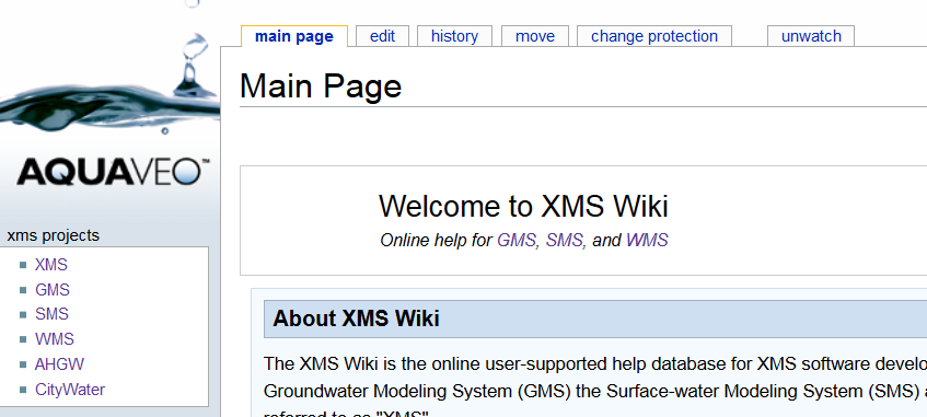
When you visit any page on the XMS Wiki, an "XMS Projects" menu is found at the top left of the page. Click on any of the products listed there to be taken to the main page for that product. Once there, click on any of the links in the Wiki Sections section on the lower right to be taken to a table of contents listing all of the pages discussing the features of that product.

Example of the XMS Wiki

At the bottom of the main page for the product, there is also a navigation template listing main topics for that product. This allows you to quickly navigate to any of those main topics.

Search Field
Example of the XMS Wiki Projects menu

Directly below the "XMS Projects" menu is a search field. If you start typing in that field, the XMS Wiki will attempt to locate a page containing what you type. To find a page about a particular product, preface the search term with that product's abbreviation, followed by a colon and the search term. For example, if you are searching for information about the bridge scour features in SMS, type "SMS:Bridge Scour" and a list of articles will appear below the search box. Simply select the desired article to be taken directly to it.

You can also enter only the search term and select the "containing…searchterm", where "searchterm" is the term you entered in the search box. This will bring up a list of pages containing the term you entered. This can be useful when you don't know what the page might be named, but you know a term that might be used on that page.

Categories

At the bottom of every page on the XMS Wiki is a list of one or more categories. This provides another way to locate information on a given topic. Simply click on the category to find a list of pages, images, and additional categories related to that topic.

Google

One option that is often overlooked is to use the power of the Google search engine. To search for pages or information on the XMS Wiki, enter "searchterm site:xmswiki.com", replacing "searchterm" with the word or words you are seeking. This tells Google to provide results only from the XMS Wiki. Click this link for an example.

Page Prefixes

Most pages on the XMS Wiki are prefaced by a product abbreviation. When reviewing search results, make sure the page you are on has the appropriate abbreviation at the beginning of the page title (e.g., "SMS:Display Options", "GMS:Display Options", "WMS:Display Options"), as similar pages may be found for various products.

Page Notices

Sometimes when searching for information or a feature, you may find pages that document obsolete or future features. These pages will have notices at the top indicating this status. There are other types of notices that may appear at the tops of pages, as well, so always be sure to read any notices that appear.

Try out these search methods today by visiting the XMS Wiki today!

Blog tags: 

Snapping Mesh Nodes to Arcs

After generating a mesh, you might notice that not all of the nodes line up along key features. There are a few ways to resolve this, but SMS 13.0 introduces a new method: the Snap Mesh to Arcs command.

In order to use the Snap Mesh to Arcs command, you must have the following:

  • 2D Mesh
  • Map coverage

Once you have the needed components, snap the nodes to an arc by doing the following:

  1. On the map coverage, draw an arc or arcs where you want to move the mesh nodes.
  2. Select the desired arcs.
  3. Make certain the correct map coverage and mesh are active in the Project Explorer.
  4. Right-click on the map coverage in the Project Explorer and select Snap Mesh to Arcs.
  5. Specify a tolerance value in the Snap Mesh to Arcs dialog.
Example of snapping mesh nodes to arcs

The command aligns the nodes in the mesh to the selected arcs in the map coverage. If no arcs are selected, this command will move nodes for all arcs in the coverage, so be certain to either select the correct arcs or make certain there are no extra arcs on the coverage.

When using the tool, it will only work with the active mesh and the active map coverage. Be certain that the correct mesh and map coverage are active in the Project Explorer.

It should be noted that not all nodes will be snapped to the selected arc. Any node that could cause instability, if moved, in the mesh will not be moved. Furthermore, nodes outside of the tolerance value will not be moved. When the nodes have been moved they cannot be moved back, therefore it might be a good idea to first use the tool on a duplicate of the target mesh then, if the results are good, rerun the tool on the target mesh.

The Snap Mesh to Arcs tool can be a useful addition to your mesh editing tools. Try it out in SMS today!

Blog tags: 

Using Display Options with Multiple UGrids

Have you experienced setting display options for an unstructured grid only to see those settings not take? In GMS, each unstructured grid (UGrid) uses its own set of display options. A common reason for display settings not appearing is selecting the wrong UGrid when you have multiple UGrids.

Changing the UGrid display settings will only affect one UGrid at a time. So it is important to make certain the correct UGrid display options are being changed.

There are three ways to reach the Display Options dialog for UGrids:

  • Display Options macro
  • Display Options command in the Display menu
  • Display Options command in the UGrid Data right-click menu in the Project Explorer
Display Options list showing multiple UGrids

Once in the Display Options dialog, check to see which UGrid is active. This is done by looking a the list on the left side of the dialog. The list on the left will indicate which By default, the display option will be set for the active UGrid. So one method to make certain you are setting display options for the correct UGrid, it to make certain that UGrid is the active UGrid in the Project Explorer before entering the Display Options dialog.

Multiple UGrids in the Project Explorer

The Display Options dialog can be used to change display settings for a UGrid that is not active. This is done by selecting the desired UGrid from the list on the left in the dialog. It should be noted that selecting a UGrid in th Display Options dialog does not cause the UGrid to become the active UGrid in GMS. So when you exit the Display Options dialog, you may need to change which UGrid is active in the Project Explorer to see the display setting changes.

It should be noted that which UGrid is active also matters when accessing the Dataset Contours Options dialog.

Hopefully, this helps clarify how to set display options in projects that have multiple UGrids. Make use of Ugrids disaply options in you project using GMS today!

Blog tags: 

Changing the Hydrograph Display in WMS

One of the more useful functions of WMS is displaying hydrographs. But did you know that WMS provide a multitude of ways to display each hydrograph?

Using the hydrograph display options allows you to alter the display of each hydrograph to better show the hydrograph data. To customize the WMS hydrograph display, right-click on the open hydrograph and select Display Options. This brings up a dialog with options to change the display for that hydrograph.

Below is a summary of the items that can be customized on each of the Display Options tabs.

Hydrograph display example
  • The General tab allows changing items such as the hydrograph title and subtitle as well as the border style and viewing style. It also allows for changing the font size. The grid lines are also controlled here to let you decide the line precision and if the x and y lines will be shown.
  • The Plot tab contains a number of present plot options to adjust how the hydrograph data is shown. Some of the options include changing to a bar graph, only displaying points, using 3d display, or selecting different line graphs.
  • The Axis tab define how x and y axis are displayed. Specifically, the values range shown on these axis can be truncated or adjusted.
  • The Font tab controls the font used for the title, subtitle, points, axis, etc.
  • The Color tab allows changing the color of the plot labels and area. A number of preset color options are also included.
  • The Style tab changes the size, style, and color of the point and lines used in the hydrograph.

Once you have set the hydrograph displays to best show off the data, you can export your hydrograph. Hydrographs can be exported either by right-clicking on them and choosing Export/Print, or by choosing the Export button from within the Display Options dialog. Export formats include JPG, PNG, and text files. Hydrographs can be printed, copied to the clipboard, or saved to a file location.

Now that you have more tools for working with hydrographs, try them out in WMS today!

Blog tags: 

Using Constant Paving Density

Starting in SMS 13.0, there is a new paving option for 2D meshes.

Paving and other mesh types, such as patching, determine the shape and size of elements (cells) when generating 2D meshes. These options are set on polygons in the Map module using the 2D Mesh Polygon Properties dialog.

Using the correct mesh type can have a large impact on your project. A good mesh type will create the correct shape and size of the mesh elements that model the physical features accurately. Selecting the wrong mesh type can add needless complexity to your mesh and cause errors in the model run.

Previous mesh type methods included patch, paving, and scalar paving density.

The pave meshing method fills a mesh polygon with equilateral, triangular elements. The new constant paving density uses the same approach as paving, but with an added component of a size and bias specified for each polygon. Size controls the target element size, while bias controls how quickly the elements transition to that size.

The following image shows the effects of changing the size and bias for a 100 x 200 rectangular mesh, with arc spacing of 5.

It should be noted that the above are merely examples to demonstrate the effect of changes in the size and bias values. For smooth transition of element size, it is recommended that the bias value be less than 0.3. Having element sizes that change too quickly can significantly impact the model run results.

As always, it is a good idea to perform a mesh quality check on the final mesh before including the mesh in your model. If problems are found in the mesh, adjust your size and bias setting then regenerate the mesh.

With the options available for mesh types, these tools should give you what you need to make the perfect mesh for your projects. Try the constant paving density option in SMS today!

Blog tags: 

Converting a 3D Dataset to a 2D Dataset

It sometimes happen where you have a fully developed 3D model in GMS and need to transfer a dataset from the 3D model to a 2D model. GMS provides a way to convert a dataset on a 3D grid to a 2D grid. From there the dataset can be exported as 2D data for use in a 2D model.

To acquire a 2D dataset from a 3D dataset, you need the following:

  • 3D grid
  • 2D grid
  • 3D dataset

To convert a 3D dataset to a 2D dataset, do the following:

  1. In the Project Explorer, select a dataset under a 3D Grid.
  2. Use the Grid menu to select the 3D Data → 2D Data command.
  3. Select option in the 3D Dataset → 2D Dataset dialog.
3D dataset to 2D dataset

The 3D Dataset → 2D Dataset dialog allows choosing which dataset to converted. By default, the dialog will use whichever 3D dataset is active in the Project Explorer. If another dataset is desired, from a MODFLOW simulation for example, you can make the change in the dialog..

The dialog also allows creating the new 2D dataset using one of the following parameters:

  • Maximum value in ij column
  • Minimum value in ij column
  • Average value in ij column
  • Sum of values in ij column
  • Highest active value in ij column
  • Value from k layer

K represents the layer number with 1 being the surface layer, and J and I representing the x and y locations of a cell (or column of cells) in the grid.

Keep in mind that one of the grids could be covering the other so if you want to observe specific data, you may need to turn off other data.

Additional additional information about converting 3D grids to other data can be found on our wiki.

Try out converting 3D datasets to 2D datasets in GMS today!

Blog tags: 

Common Installation Issues with XMS

Are you having trouble installing GMS, SMS, or WMS? Here are three common installation issues, and how to overcome them.

Virtual Machines

The main issues when using virtual machines is selecting the correct type of installation. Single-user locks are not compatible with virtual environments. If you are trying to install XMS with a single-user lock and a virtual machine is detected, XMS will not install. You will need a network lock to get around this issue. Network locks are designed to be used with virtual machines. Single-user locks are not capable of being used as a network lock.

Firewalls and User Permissions

Sometimes, a good password will fail to install XMS, This is because your computer actually needs to contact our servers to verify the authenticity of the password. When an internet error comes up, it's typically related to a firewall, user permissions, or antivirus software blocking the connection to our servers.

Try one of these solutions to resolve this issue:

  • Whitelist which ever XMS program you are trying to install and the registration wizard.
  • Temporarily disable the firewall/antivirus software.

Note that firewalls are typically something each company's IT department handles.

If you are running Windows 8 or 10, and you are not running in a virtual environment, then the issue could be caused by a Windows feature called Hyper-V. Disabling Hyper-V can resolve the problem. You can find instructions on how to disable Hyper-V by reading this article.

Hardware locks

When installing a hardware lock, be sure to have your drivers installed and running before attempting to register the lock. Additionally, please also ensure that the lock is plugged into the computer at the time you are attempting to register. (Note that as a security measure, the reburn cannot take place remotely.) For instructions on how to install your specific type of hardware lock please visit our page here.

Feel free to contact our technical support team at support@aquaveo.com for more individual help in troubleshooting any of these problems. Please recognize that Aquaveo technical support can only help troubleshoot individual machine issues to a certain point.

Blog tags: 

How to Generate a Flood Depth Raster

After running your model, such as SRH-2D, you will have a water surface elevation (WSE) dataset. Did you know that, starting in SMS 13.0, you can use the WSE dataset to create a raster showing the flood depths?

SMS can create a flood depth raster by using the WSE solution dataset at a specific time step and comparing it to the initial elevation data. Using both of these datasets, it can then generate a raster that shows the flooded areas for a specific time step.

In order to create a flood depth raster your project will need a WSE solution dataset and an elevation raster. Once you have a raster:

  1. Select the desired time step for your WSE solution dataset.
  2. Right-click on the raster and select Convert To | Flood Depths.
  3. In the Select Geometry and Dataset dialog, select a geometry containing your WSE solution dataset. The selected geometry can be either a 2D mesh or a 2D scatter set.
  4. Next select the WSE solution dataset.
  5. Click OK to close the Select Geometry and Dataset dialog, which will launch the Save As dialog.
  6. Creating a name for your raster and click Save. (Note that the file should be saved as a "GeoTIFF Files (*.tif)".
  7. Hide the mesh and elevation raster to be able to view your new flood depth raster.

It should be noted that it may take a few minutes for the flood depth raster to be generated depending on the available processing power of your machine. Since a raster file is saved during the process, the file is available for use in other applications if desired. Coordinate data is saved with the file.

Now that you know to create flood depth rasters, try using them in your SRH-2D projects in SMS.

Blog tags: 

Changing an Existing Model to be a Predictive Model

When you have a completed GMS model, you can use that same model to create a predictive model. A predictive model is used to make predictions based on hypothetical future scenarios. For example, you may need to create a model that predicts if an aquifer will experience strain with an increased population drawing from the aquifer in the model area.

Groundwater model

In general, a predictive model is created by using an existing model, then altering an aspect of that model based on the hypothesis. You then run the model again and compare your results with your prediction. Any version of MODFLOW, or any of the other available numeric models in GMS, can be used to create a predictive model.

One method of setting up a predictive model might be as follows:

  1. Create and run a steady state model
  2. Calibrate the model to reduce error in the predictive model
  3. Set the transient settings to a future date
  4. Run the transient model

It is important for you to have an expectation of the outcome of the model run so that you can compare the results with that expectation. When the model run is completed, carefully review the model run results to determine the accuracy of the predictions. When creating a predictive model, you can make use of stochastic analyses.

If the predictive model seems to be far outside of your expectations, then you will need to troubleshoot the existing model before running the predictive model. Using a poorly developed existing model often leads to issues in the predictive model. Make certain the existing model has been well calibrated to closely match the field-observed values. If possible, calibrate the existing model to multiple sets of observation data before creating a predictive model.

Now that you know some of the principles in developing a predictive model, creating your own predictive model in GMS today!

Blog tags: 

Tips for Managing Cross Sections in WMS

Cross sections are commonly used in 1D models within WMS. Here we discuss a few things to help you better model using cross sections.

When you create cross sections in WMS, you must create them on "1D-Hyd Cross Section" coverage. You then create the arcs on this coverage to represent the cross sections.There are a few things you should remember when setting up your cross sections:

  • Cross sections should be located at fairly frequent intervals along the river. This makes sure the characterization of the stream channel and floodplain flow and capacity is accurate, which gives you better results.
  • You should place cross sections especially at locations of significant change, where levees begin and end, at hydraulic structures, and around stream junctions.
  • The cross section arcs should generally stretch from one side of the river floodplain to the other.
  • They should be generally perpendicular to the river arc where they cross.
  • Cross section arcs should not cross each other.
Hydraulic Model Example with Cross Sections

In addition to the above, each cross section should have the following required information:

  • River name
  • Reach name
  • River station
  • Description
  • Station–elevation data
  • Downstream reach lengths
  • Manning’s n values
  • Main channel bank stations
  • Contraction and expansion coefficients

It is recommended that the station number be visible on the map view to make the cross sections more identifiable. This can be enabled in the Display Options dialog. When numbering stations, they must be in ascending numerical order from downstream to upstream. If changes are made, be sure to renumber the stations.

Converting an arc into a cross section arc can be done automatically or manually. You can automatically do it by taking the following steps:

  1. Define or import a TIN.
  2. Create an area property coverage, a centerline coverage, and a 1D-Hyd cross section coverage.
  3. Use the Extract Cross Section command to extrude the cross sections from the 2D arcs.

To manually create a cross section arc:

  1. Double-click on the cross section arc and select Assign Cross Section.
  2. Define the various elevations and data as desired.

Try out these tips and procedures today in the WMS Community Edition!

Blog tags: 

Pages