Using Internal Sinks and Links in SRH-2D
By aquaveo on July 17, 2019Do you have an SRH-2D project that requires placing a drain inside the mesh? Or perhaps you have two seperate meshes in your project where you need to have water flowing between them? Both of these scenarios can be resolved by respectively using the internal sink and link boundary conditions.
Internal Sink Boundary Condition
The internal sink boundary condition is assigned to an arc on an SRH-2D boundary condition map coverage. Unlike an inflow or outflow boundary condition, an internal sink is assigned to an arc that is inside the mesh boundaries.
An internal sink can simulate wells, drains or other points of outflow. It can also simulate a source by specifying a negative number for the flow.
It should be noted that an internal sink boundary condition should not be used as a model’s primary source of inflow or outflow. Inflow and outflow boundary conditions should be placed on the mesh boundary.
Links
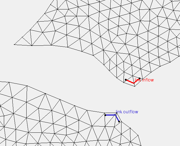
Link boundary conditions can be used to simulate moving water between two different meshes or two different areas of the same mesh. Links can sometimes be used to make a simple representation of a pipe or similar structure connecting two areas.
Links are made by making two arcs on an SRH-2D boundary condition coverage. Both arcs are selected when assigning the Link property type. One arc should be assigned as the link inflow boundary condition and the other arcs should be assigned as the link outflow.
It should be noted that link boundary conditions should not be used to model culverts or other such structures. Also, link boundary conditions should not be used as the primary inflow or outflow source for a project.
Now that you know a little more about using internal sink and link boundary conditions, try using them in your SRH-2D projects in SMS.