Splitting UGrid Layers
By aquaveo on May 8, 2019Have you been working with a project in GMS only to discover that the project’s 3D unstructured grid (UGrid) needs to include another layer? Fortunately, it’s rare that a UGrid needs to have another layer, but every once in a while a layer needs to be added to an existing UGrid. GMS provides a way to divide UGrid layers quickly.
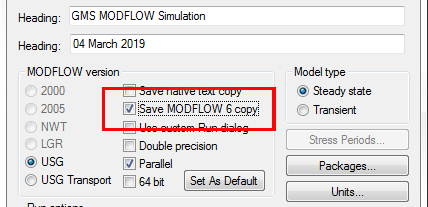
One thing to note: whenever a UGrid is changed—such as with adding a new layer—the existing MODFLOW simulation attached to the UGrid will be removed. It is therefore best to make certain the UGrid is correct—including having the necessary number of layers—before building the MODFLOW simulation.
In order to add a new layer to an existing Ugrid, do the following:
- Using the Select Cell tool, select a cell on the layer you want to split.
- Right-click on the selected cell and select the Split Layer command to start the process of dividing the UGrid layer.
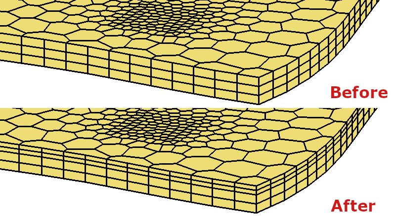
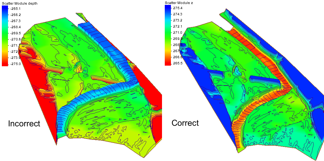
When GMS finishes processing, it creates a new UGrid with the additional layer, leaving the original UGrid intact. The layer to which the selected cell belonged is divided into two layers on the new UGrid. GMS averages the distance between the top and bottom of the layer, then divides the layer equally to create the two new layers. It is recommended to carefully review the new UGrid to check for any unintended anomalies.
As mentioned above, any MODFLOW simulations contained in the original UGrid are not copied to the new UGrid. A new MODFLOW simulation must be created for the new UGrid.
Another option is to create a new UGrid with the additional layer and leave the existing UGrid as is. This option is best if you need to finely control the layer elevations.
For adding layers to complicated UGrids, you may want to consider using Aquaveo’s consulting services.
Now that you’ve seen the basics of splitting a UGrid layer, try it out in GMS today!