Visualizing Meteorological Data
By aquaveo on August 1, 2018Do have rainfall data you would like to visualize in WMS? Inside WMS there are a couple tools to make your rainfall data visually interesting.
After you have imported your precipitation data, such as NEXRAD data, you can adjust your display options and/or create an animation.
Adjusting the Display Options
- Use the Display | Display Options command to open the Display Options dialog.
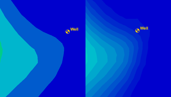
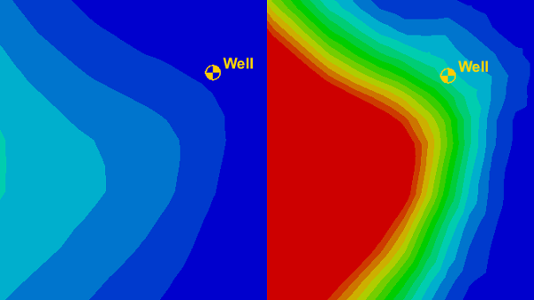
- Adjust your display options to show the data you want captured. It is recommended to turn on the Contours options.
- If using the Contours option, right-click on your rainfall dataset under 2D Grid Data and select Contour Options to open the Contour Options dialog.
- Adjust the contour method and interval to best display your rainfall data.
- With the down arrow key on the keyboard, step through the time steps in the properties window on the right sidebar to see how the precipitation varies.
Creating an Animation Loop
- Select your rainfall dataset in the 2-D Grid Module. The selected dataset will be used to create the film loop and can be cumulative or incremental. View incremental rainfall datasets in the same way as cumulative datasets.
- Select the Data | Film Loop command to open the Film Loop Setup Wizard. This wizard needs to be opened with the 2-D Grid Module active in order to have access to the meteorological data options.
- The first step in the Film Loop Setup wizard is essentially the same as creating any other animation through WMS. Select the location where the animation file will be saved and the type of film loop to generate.
- The second step of the Film Loop Setup wizard is to set the desired time step options for the rainfall data.
- The final step is where you will finalize the display options of the animation, and click Finish.
- WMS will take a few moments to create and save the animation file. The animation will start playing as soon as the saving process is complete.
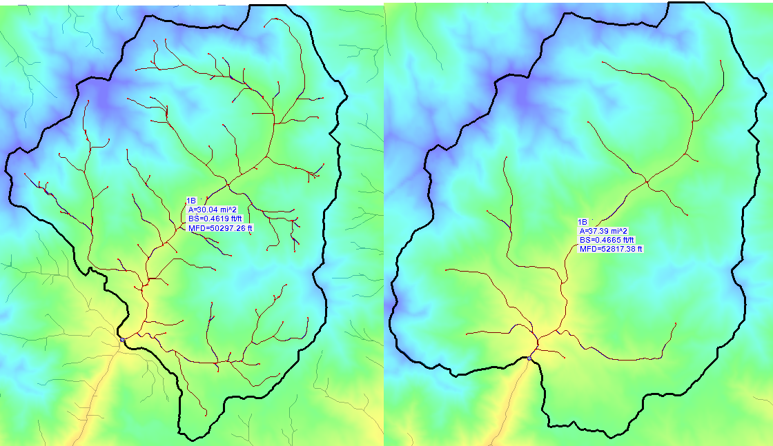
When all is done, you can view your animation using the AVI play provided with the WMS installation, or you can use another application, such as GoogleEarth. The animation will display the movement of the storm through the selected time steps.
Try visualizing meteorological data in WMS today!