Performing a Silent Install of XMS
By aquaveo on October 10, 2018This blog post provides information on older password and hardware lock configurations.
Information on new local and flex codes may be found here.
Are you an IT administrator needing to perform a silent install of GMS, SMS, or WMS in a classroom or office? Some classrooms and offices have multiple students or employees changing machines regularly. Non-administrator users are often unable to change the licensing password, lock, or server when these license settings are stored in the global area of the registry. Because of this, we changed the license settings so they are now stored in the user area of the registry. This means that each user account requires this to be setup.
This silent install (or quiet install) workaround requires each user to have the rights to modify the registry. If registry access is restricted, a network administrator can do this by opening the Group Policy Management Editor and creating a startup script that automatically runs the batch file whenever the computer is restarted.
Note: Editing the Registry in Windows is a very advanced administration step. Please always create a backup of the Registry before making changes.
It can be a burden have to manually update the network lock server address in HKEY_CURRENT_USER for each user on each computer. The silent install process is simplified by creating a Windows Registry file that contains the license information and a batch file that can be executed to insert the registry information and launch WMS. The batch file automatically updates the registry for the user and then opens the WMS application. This is the safest way to edit the registry key, as well. The batch file can then be placed on each computer that needs to be updated, and the individual users can execute it as needed.
This workaround uses WMS as an example. This information also applies to GMS and SMS. You can see an example of a registry file in step 1 and the batch file in step 2, below.
- Create a file, “Netenble.001.reg”, as follows, replacing "license" with the name or IP address of the network lock server. For example, if the network lock server was at 127.0.0.27, you would use “127.0.0.27”:
Windows Registry Editor Version 5.00M


[HKEY_CURRENT_USER\Software\EMRL\WMS]

"Netenble.001"="license"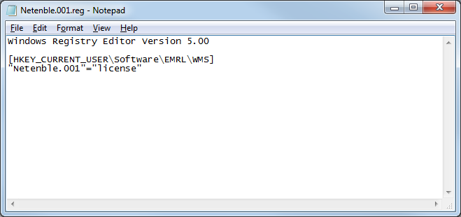
Note: This information was created using Windows 7. Because different Windows versions can have different REG file formats, we recommend you install WMS on one machine, register it to the correct network lock server, then export the [HKEY_CURRENT_USER\Software\EMRL\WMS] registry key. Open the registry file in the text editor and remove every line except those similar to those shown in the image above, and save the file as “Netenble.001.reg”. -
Create a file, “wms11.bat”, that will update the registry and start WMS:
reg import Netenble.001.reg

wms.exe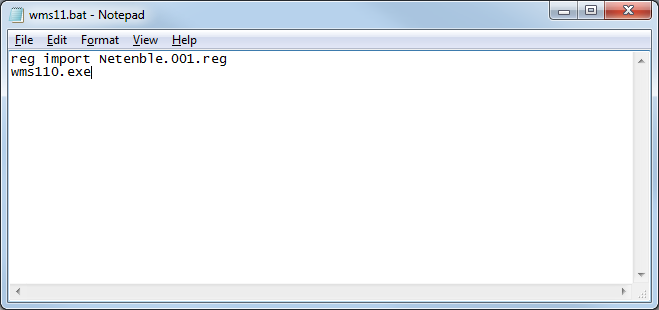
- Place these two files in the WMS folder in the image that will be distributed to the affected computers. For example, for the 64-bit version of WMS 11.0, the default location for the folder is “C:\Program Files\WMS 11.0 64-bit\”.
- Create a desktop shortcut to the batch file for the convenience of the user. If doing this via a startup script in the Group Policy Management Editor, this step can be skipped.
This silent install workaround can save you significant time as a network administrator. Try it out today!