Running MODFLOW Outside of GMS
By aquaveo on April 20, 2022Do you have a MODFLOW project you created in GMS, but realize you need to run MODFLOW outside of GMS? This is sometimes necessary if you have a very specific need for your project that can only be accomplished by modifying the exported files before running the MODFLOW simulation. This does not happen often, but when you do encounter a situation where you need to run MODFLOW outside of GMS, do the following:
- Open the MODFLOW Global Options and make certain that the Save as Native Text option has been turned on. This is necessary to generate files for your project that you can edit. With the native text option turned on, saving your project will generate the native text files.
- One you have the native text files generated, you can then edit the files manually using a text editor. GMS will create a separate directory with the native MODFLOW files. This directory will typically be the project name with "_text" appended to it. For example, if the project is named "Aquifer", the directory will be named "Aquifer_text". Keep these files together.
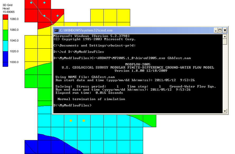
- To run the native files, use either a command line with a DOS prompt or a batch file. See guidance for how to do this on USGS's website.
- After you have successfully run your MODFLOW simulation, import back into GMS to visualize the results and perform additional analyses using the tools in GMS. You will need to start by importing either the NAM file or MFN file. These files contain a directory for the other files in the MODFLOW project and how they should be opened. It is important to keep all of the MODFLOW files together in the same directory. Having only the NAME or MFN file will not be enough to open the MODFLOW project. Files for the packages used with the project will typically have a file extension that matches the package. For example, the Wells package will have the extension "*.wel".
Running the native files outside of GMS can be used to validate results of a GMS model or to add custom parameters not available in GMS. However, Aquaveo may not be able to provide technical support for simulations that have been extensively modified outside of the GMS application.
Knowing how to run MODFLOW outside of GMS can give you more options for modeling with GMS. Try out GMS 10.6 today!